Day 1 – Spatial & Spatio-Temporal Modelling

Author

Olatunji Johnson

Overview

Today we introduce modern geostatistical modelling using inlabru, covering:

Spatial models
- Binomial likelihood (prevalence)
- Poisson likelihood (case counts)
- SPDE spatial random fields
- Prediction surfaces
- Exceedance probabilities
Spatio-temporal models
- Handling time-indexed disease data
- RW1/RW2 temporal structure
- Spatio-temporal Gaussian fields
- Predicting in time and space

These form the foundation for Days 2 and 3.

============================================================

PART A — Spatial models

============================================================

1. Load data

The data used for Day 1 are a simulated malaria prevalence dataset from Nigeria. If malaria is of particular interest in your research, you can download real datasets from the DHS website. Malaria data can be obtained either from prevalence surveys or from hospital records.

When derived from prevalence surveys, the data can be treated as binomial, since you observe the number of individuals surveyed and the number who tested positive. When obtained from hospital records, the data typically consist of counts of positive malaria cases at specific locations and can be modelled as Poisson data.

Code

library(tidyverse)
library(INLA)
library(inlabru)
library(ggplot2)
library(sf)
library(stars)
# library(rnaturalearth)
# library(rnaturalearthdata)
library(geoR)

# nga_admin1 <- ne_states("Nigeria", returnclass = "sf") %>%
# st_transform(32632)

nga_admin1 <- st_read("data/nga_shapefile.shp")

Reading layer `nga_shapefile' from data source 
  `/home/olatunji-johnson/Documents/Manchester Job/Teaching/Courses/Nigeria_2026/rcode/FUTA/data/nga_shapefile.shp' 
  using driver `ESRI Shapefile'
Simple feature collection with 37 features and 121 fields
Geometry type: MULTIPOLYGON
Dimension:     XY
Bounding box:  xmin: -198992.3 ymin: 472813 xmax: 1117766 ymax: 1537228
Projected CRS: WGS 84 / UTM zone 32N

Code

spatial_binom <- read_csv("data/spatial_binomial_data.csv")
spatial_pois  <- read_csv("data/spatial_poisson_data.csv")

2. Convert to sf for mapping

We need an sf layer to overlay boundaries, plot points, and feed coordinates into SPDE meshes.

Code

spatial_binom_sf <- spatial_binom %>%
  st_as_sf(coords = c("utm_x", "utm_y"), crs = 32632)
spatial_pois_sf <- spatial_pois %>%
  st_as_sf(coords = c("utm_x", "utm_y"), crs = 32632)

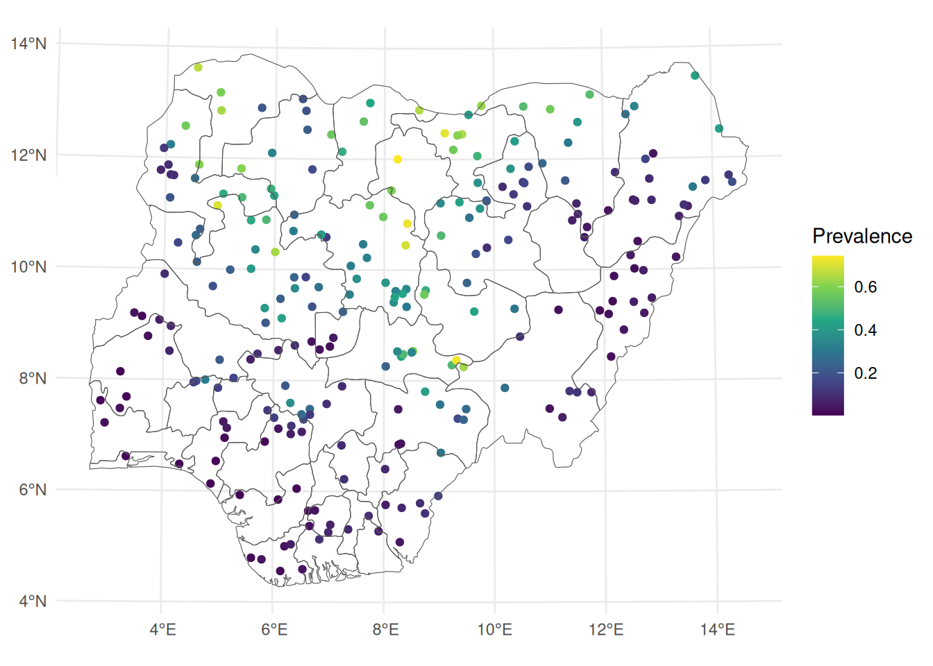
3. Visualise sampling locations

This helps confirm:

UTM conversion is correct
Points sit inside Nigeria
Prevalence has spatial structure

Code

ggplot() +
geom_sf(data = spatial_binom_sf, aes(colour = prevalence_true)) +
geom_sf(data = nga_admin1, fill = NA) +
scale_colour_viridis_c(name="Prevalence") +
theme_minimal()

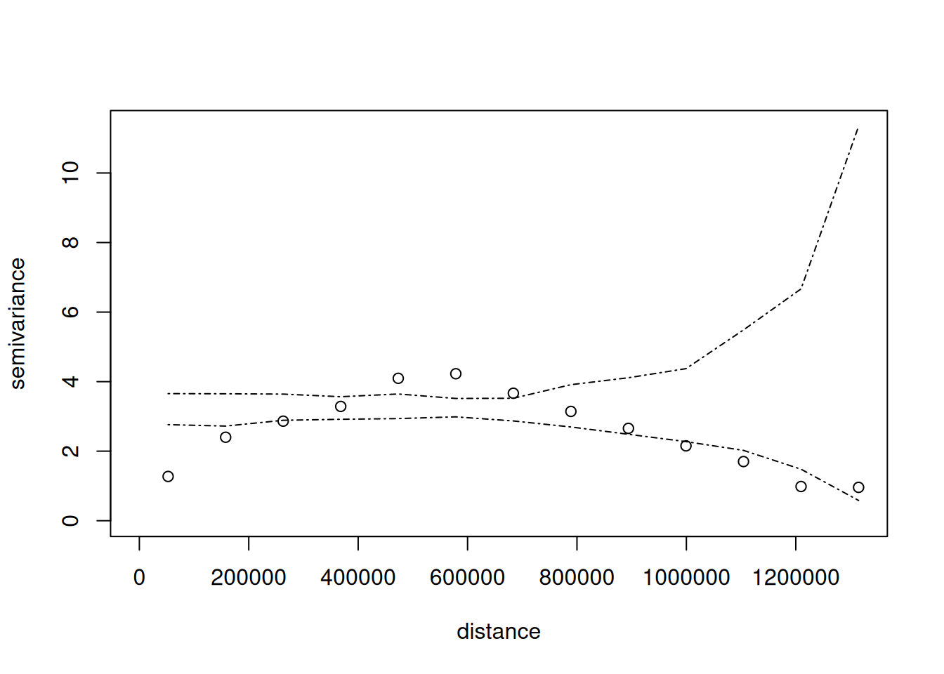
4. Variogram

Before proceeding to spatial modelling, there is a need to check for the evidence of spatial correlation in the residual. Variagram can be used to achieve this.

Code

non_spatial_fit <- glm(prevalence_true ~ elevation + ndvi + urban, data = spatial_binom, weights = n_tested)
resid <- residuals(non_spatial_fit)
spatial_binom$resid <-resid
geo_data <- as.geodata(obj = spatial_binom, coords.col=2:3, data.col=ncol(spatial_binom))
vari <- variog(geo_data)

variog: computing omnidirectional variogram

Code

vari.mc <- variog.mc.env(geo_data, obj.variog=vari, nsim=1000)

variog.env: generating 1000 simulations by permutating data values
variog.env: computing the empirical variogram for the 1000 simulations
variog.env: computing the envelops

Code

plot(vari, envelope.obj=vari.mc)

We can see that there is an evidence of spatial correlation because the empirical semi-variogram for the data does not completely lie inside the envelopes, especially at smaller distances.

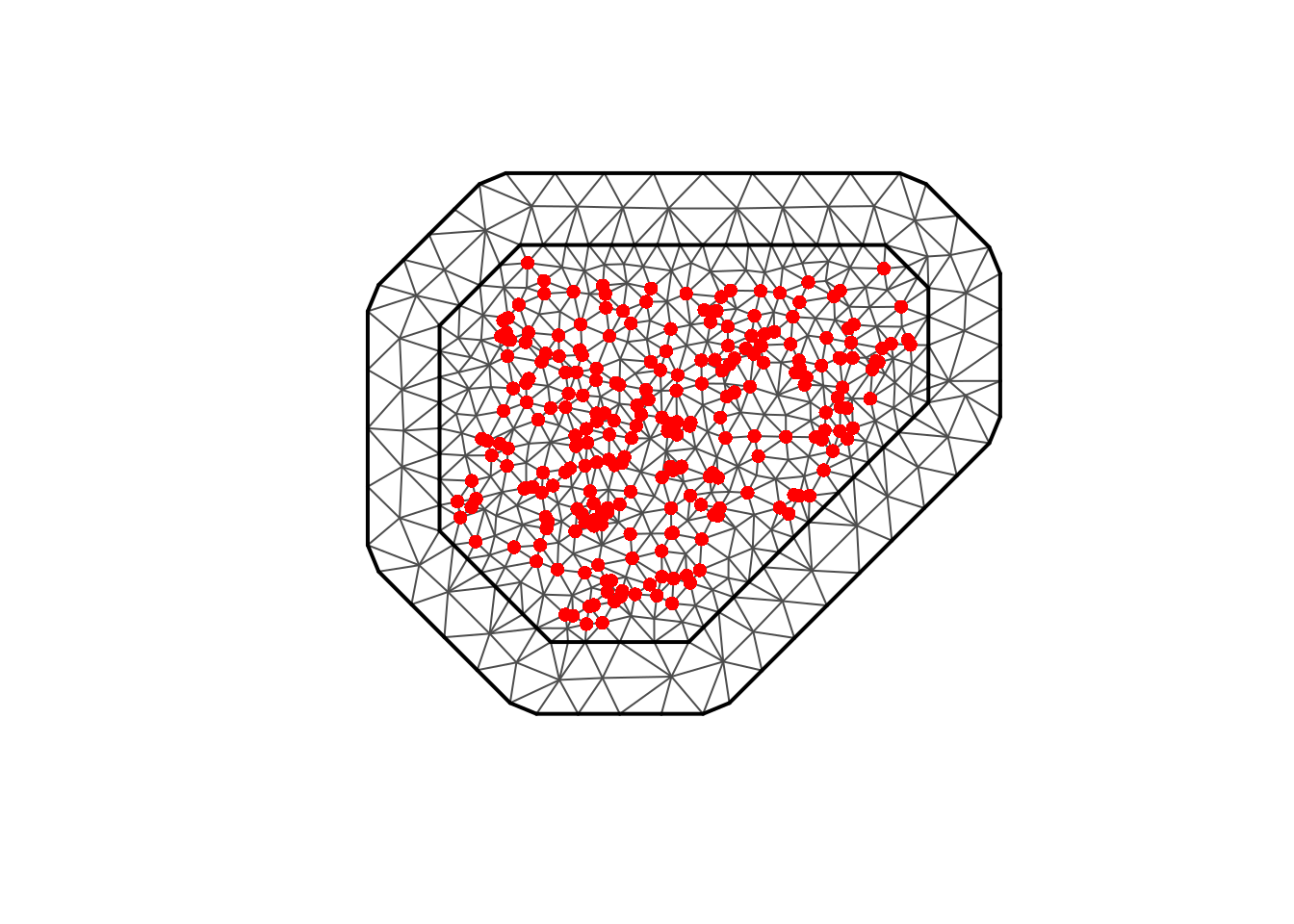
5. Build the SPDE mesh

The mesh defines the geometry on which the latent spatial field is approximated.

Code

coords <- st_coordinates(spatial_binom_sf)

mesh <- inla.mesh.2d(
loc = coords,
max.edge = c(100000, 200000), # inner and outer triangle sizes
cutoff = 20000,  # merge points closer than 20km
offset = c(50000, 200000)  # extend mesh beyond convex hull
)

plot(mesh)
points(coords, col="red", pch=16)

A finer mesh → more accurate, more expensive.
A coarser mesh → faster, less precise.
We balance cost vs smoothness.

6. SPDE model (PC priors)

Penalised complexity (PC) priors make spatial models robust and interpretable.

Code

spde <- inla.spde2.pcmatern(
mesh = mesh,
prior.range = c(300000, 0.5),
prior.sigma = c(1.0, 0.01)
)

7. Spatial BINOMIAL model

The model is:

\[logit(pi)=\beta_0+\beta_1 elevation_i+ \beta_2ndvi_i+ \beta_3 urban_i+ S(s_i)\]

Where \(S(\mathbf{s})\) is a spatial Gaussian field.

Code

components_binom <- ~
Intercept(1, model="linear") +
beta_elev(elevation, model="linear") +
beta_ndvi(ndvi, model="linear") +
beta_urban(urban, model="linear") +
field(geometry, model = spde)

lik_binom <- like(
family="binomial",
data=spatial_binom_sf,
formula = n_pos ~ Intercept + beta_elev + beta_ndvi + beta_urban + field,
Ntrials = n_tested
)

#| cache: true
fit_binom <- bru(components_binom, lik_binom)
summary(fit_binom)

inlabru version: 2.13.0.9024 
INLA version: 25.12.02 
Latent components:
Intercept: main = linear(1)
beta_elev: main = linear(elevation)
beta_ndvi: main = linear(ndvi)
beta_urban: main = linear(urban)
field: main = spde(geometry)
Observation models:
  Model tag: <No tag>
    Family: 'binomial'
    Data class: 'sf', 'tbl_df', 'tbl', 'data.frame'
    Response class: 'numeric'
    Predictor: n_pos ~ Intercept + beta_elev + beta_ndvi + beta_urban + field
    Additive/Linear/Rowwise: TRUE/TRUE/TRUE
    Used components: effect[Intercept, beta_elev, beta_ndvi, beta_urban, field], latent[] 
Time used:
    Pre = 1.41, Running = 1.78, Post = 0.338, Total = 3.53 
Fixed effects:
             mean    sd 0.025quant 0.5quant 0.975quant   mode kld
Intercept  -3.464 0.779     -5.034   -3.452     -1.965 -3.453   0
beta_elev  -0.003 0.001     -0.006   -0.003      0.000 -0.003   0
beta_ndvi   5.350 1.305      2.796    5.340      7.962  5.341   0
beta_urban  0.456 0.059      0.341    0.456      0.572  0.456   0

Random effects:
  Name    Model
    field SPDE2 model

Model hyperparameters:
                    mean       sd 0.025quant 0.5quant 0.975quant     mode
Range for field 2.79e+05 4.70e+04   2.01e+05 2.74e+05   3.86e+05 2.62e+05
Stdev for field 1.12e+00 1.34e-01   8.90e-01 1.11e+00   1.42e+00 1.08e+00

Marginal log-Likelihood:  -935.76 
 is computed 
Posterior summaries for the linear predictor and the fitted values are computed
(Posterior marginals needs also 'control.compute=list(return.marginals.predictor=TRUE)')

8. Spatial POISSON model

Often used for malaria case counts or incidence.

Model: \[\log(\lambda_i)= \beta_0 + \beta_1 X_i + S(s_i)\]

Code

components_pois <- ~
Intercept(1, model="linear") +
beta_elev(elevation, model="linear") +
beta_ndvi(ndvi, model="linear") +
beta_urban(urban, model="linear") +
field(geometry, model = spde)

lik_pois <- like(
family="poisson",
data=spatial_pois_sf,
formula = cases ~ Intercept + beta_elev + beta_ndvi + beta_urban + field
)

#| cache: true
fit_pois <- bru(components_pois, lik_pois)
summary(fit_pois)

inlabru version: 2.13.0.9024 
INLA version: 25.12.02 
Latent components:
Intercept: main = linear(1)
beta_elev: main = linear(elevation)
beta_ndvi: main = linear(ndvi)
beta_urban: main = linear(urban)
field: main = spde(geometry)
Observation models:
  Model tag: <No tag>
    Family: 'poisson'
    Data class: 'sf', 'tbl_df', 'tbl', 'data.frame'
    Response class: 'numeric'
    Predictor: cases ~ Intercept + beta_elev + beta_ndvi + beta_urban + field
    Additive/Linear/Rowwise: TRUE/TRUE/TRUE
    Used components: effect[Intercept, beta_elev, beta_ndvi, beta_urban, field], latent[] 
Time used:
    Pre = 1.01, Running = 2.22, Post = 0.335, Total = 3.56 
Fixed effects:
             mean    sd 0.025quant 0.5quant 0.975quant   mode kld
Intercept   0.530 0.617     -0.661    0.523      1.766  0.523   0
beta_elev  -0.001 0.002     -0.004   -0.001      0.002 -0.001   0
beta_ndvi   1.432 0.731     -0.063    1.449      2.829  1.448   0
beta_urban  0.747 0.082      0.587    0.747      0.909  0.747   0

Random effects:
  Name    Model
    field SPDE2 model

Model hyperparameters:
                    mean      sd 0.025quant 0.5quant 0.975quant     mode
Range for field 1.34e+05 3.7e+04   7.56e+04 1.29e+05   2.20e+05 1.19e+05
Stdev for field 8.23e-01 9.4e-02   6.54e-01 8.18e-01   1.02e+00 8.07e-01

Marginal log-Likelihood:  -631.40 
 is computed 
Posterior summaries for the linear predictor and the fitted values are computed
(Posterior marginals needs also 'control.compute=list(return.marginals.predictor=TRUE)')

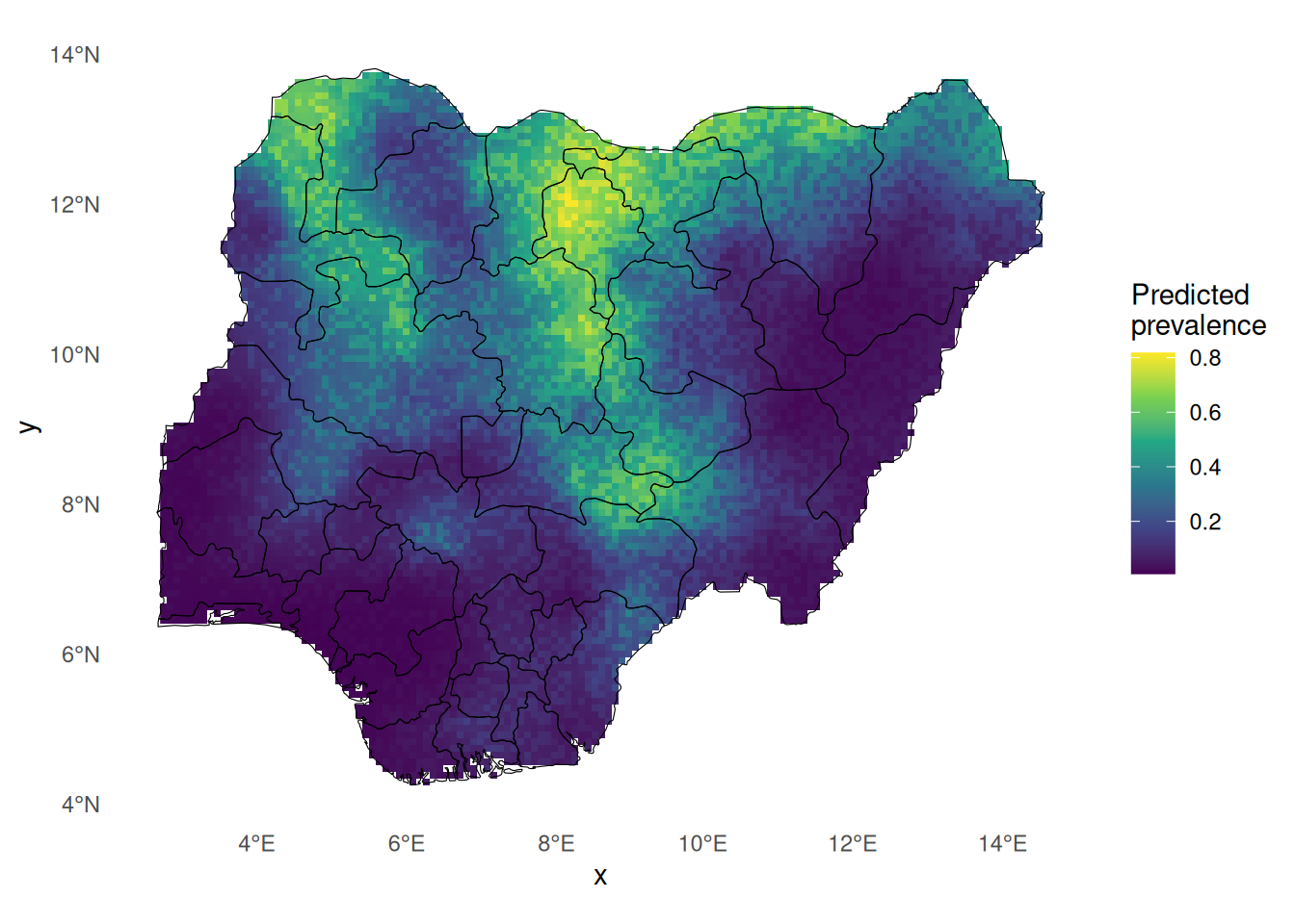
9. Predictive surfaces (binomial example)

Code

pred_grid <- read_csv("data/prediction_grid_utm.csv") %>%
st_as_sf(coords=c("utm_x","utm_y"), crs=32632)

pred_binom <- predict(
fit_binom,
newdata = pred_grid,
formula = ~ plogis(Intercept + beta_elev + beta_ndvi + beta_urban + field),
n.samples = 1000
)

Rasterise:

Code

pred_binom_r <- st_rasterize(pred_binom["mean"], dx=10000, dy=10000)
pred_binom_r <- pred_binom_r[st_union(nga_admin1)]

Plot:

Code

ggplot() +
  geom_stars(data=pred_binom_r, na.rm = TRUE) +
  geom_sf(data=nga_admin1, fill=NA, color = "black") +
  coord_sf() +
  scale_fill_viridis_c(name = "Predicted\nprevalence", na.value = NA) +
  theme_minimal() +
  theme(
    panel.background = element_rect(fill = "white", colour = NA),
    plot.background  = element_rect(fill = "white", colour = NA),
    panel.grid       = element_blank()
  )

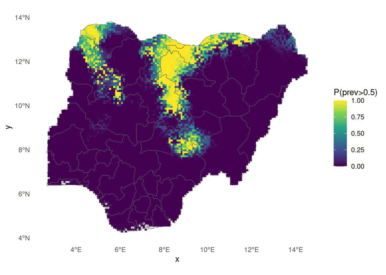
10. Exceedance probability (binomial)

Goal:

\[P(prevalence>0.5∣data)\]

Code

exc_samples <- generate(
fit_binom,
newdata = pred_grid,
formula = ~ plogis(Intercept + beta_elev + beta_ndvi + beta_urban + field),
n.samples = 1000
)

pred_binom$exc_prob <- rowMeans(exc_samples > 0.5)

Map:

Code

exc_r <- st_rasterize(pred_binom["exc_prob"], dx=10000, dy=10000)
exc_r <- exc_r[st_union(nga_admin1)]

ggplot() +
  geom_stars(data=exc_r, na.rm = TRUE) +
  scale_fill_viridis_c(name="P(prev>0.5)", limits=c(0,1), na.value = NA) +
  geom_sf(data=nga_admin1, fill=NA) +
  theme_minimal() + 
  theme(
    panel.background = element_rect(fill = "white", colour = NA),
    plot.background  = element_rect(fill = "white", colour = NA),
    panel.grid       = element_blank()
  )

============================================================

PART B — Spatio-Temporal Modelling ============================================================

We now extend:

\[S(s)⟶S(s,t)\]

A common structure:

Spatial effect: SPDE
Temporal effect: random walk (RW1 or RW2)
Interaction: separable \(S(s,t)=S_s(s)+S_t(t)\)

Code

st_binom <- read_csv("data/spatiotemporal_binomial_data.csv") %>%
  st_as_sf(coords=c("utm_x","utm_y"), crs=32632)

head(st_binom)

Simple feature collection with 6 features and 10 fields
Geometry type: POINT
Dimension:     XY
Bounding box:  xmin: 336995.7 ymin: 1047442 xmax: 336995.7 ymax: 1047442
Projected CRS: WGS 84 / UTM zone 32N
# A tibble: 6 × 11
   site  time     S gamma_t elevation  ndvi urban n_tested n_pos prevalence_true
  <dbl> <dbl> <dbl>   <dbl>     <dbl> <dbl> <dbl>    <dbl> <dbl>           <dbl>
1     1     1 0.266   2.12       228. 0.305     0       63    51           0.774
2     1     2 0.266   1.50       228. 0.305     0       65    43           0.649
3     1     3 0.266   0.381      228. 0.305     0      119    52           0.376
4     1     4 0.266   0.286      228. 0.305     0      191    72           0.354
5     1     5 0.266   0.168      228. 0.305     0      180    50           0.327
6     1     6 0.266   0.207      228. 0.305     0      155    52           0.336
# ℹ 1 more variable: geometry <POINT [m]>

Should contain:

time
n_tested, n_pos
covariates
UTM coordinates

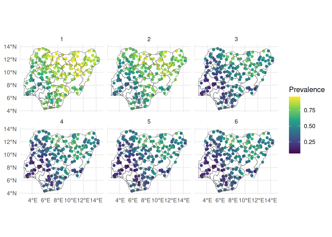
11. Mapping the spatio-temporal empirical prevalence

Code

ggplot() +
geom_sf(data = st_binom, aes(colour = prevalence_true)) +
  facet_wrap(~time)  + 
geom_sf(data = nga_admin1, fill = NA) +
scale_colour_viridis_c(name="Prevalence") +
theme_minimal()

12. Spatio-temporal components - sum of a purely spatial and a purely temporal trend.

Use: - RW1 for time - SPDE for space - Additive interaction

Code

components_st <- ~
Intercept(1, model="linear") +
beta_elev(elevation, model="linear") +
beta_ndvi(ndvi, model="linear") +
beta_urban(urban, model="linear") +
time(time, model="rw1") +
field(geometry, model = spde)

Likelihood:

Code

lik_st <- like(
family="binomial",
data = st_binom,
formula = n_pos ~ Intercept + beta_elev + beta_ndvi + beta_urban +
time + field,
Ntrials = n_tested
)

Fit:

Code

fit_st_binom <- bru(components_st, lik_st)
summary(fit_st_binom)

inlabru version: 2.13.0.9024 
INLA version: 25.12.02 
Latent components:
Intercept: main = linear(1)
beta_elev: main = linear(elevation)
beta_ndvi: main = linear(ndvi)
beta_urban: main = linear(urban)
time: main = rw1(time)
field: main = spde(geometry)
Observation models:
  Model tag: <No tag>
    Family: 'binomial'
    Data class: 'sf', 'tbl_df', 'tbl', 'data.frame'
    Response class: 'numeric'
    Predictor: n_pos ~ Intercept + beta_elev + beta_ndvi + beta_urban + time + field
    Additive/Linear/Rowwise: TRUE/TRUE/TRUE
    Used components: effect[Intercept, beta_elev, beta_ndvi, beta_urban, time, field], latent[] 
Time used:
    Pre = 0.963, Running = 2.25, Post = 0.247, Total = 3.46 
Fixed effects:
             mean    sd 0.025quant 0.5quant 0.975quant   mode kld
Intercept  -0.261 0.332     -0.909   -0.263      0.399 -0.263   0
beta_elev  -0.002 0.001     -0.003   -0.002     -0.001 -0.002   0
beta_ndvi   1.775 0.591      0.590    1.781      2.926  1.781   0
beta_urban  0.525 0.028      0.470    0.525      0.580  0.525   0

Random effects:
  Name    Model
    time RW1 model
   field SPDE2 model

Model hyperparameters:
                       mean       sd 0.025quant 0.5quant 0.975quant     mode
Precision for time 4.49e+00 2.65e+00   1.25e+00 3.88e+00   1.13e+01 2.85e+00
Range for field    1.73e+05 2.65e+04   1.28e+05 1.71e+05   2.32e+05 1.65e+05
Stdev for field    6.52e-01 5.20e-02   5.57e-01 6.50e-01   7.61e-01 6.44e-01

Marginal log-Likelihood:  -3963.37 
 is computed 
Posterior summaries for the linear predictor and the fitted values are computed
(Posterior marginals needs also 'control.compute=list(return.marginals.predictor=TRUE)')

13. Spatio-temporal components - Inseparable covariance function

Use: - Exchageable for time - SPDE for space - interaction

Code

components_st2 <- ~
Intercept(1, model="linear") +
beta_elev(elevation, model="linear") +
beta_ndvi(ndvi, model="linear") +
beta_urban(urban, model="linear") +
field(geometry, model = spde, group = time, control.group=list(model="iid")) #?control.group

Likelihood:

Code

lik_st2 <- like(
family="binomial",
data = st_binom,
formula = n_pos ~ Intercept + beta_elev + beta_ndvi + beta_urban + field,
Ntrials = n_tested
)

Fit:

Code

fit_st_binom2 <- bru(components_st2, lik_st2)
summary(fit_st_binom2)

inlabru version: 2.13.0.9024 
INLA version: 25.12.02 
Latent components:
Intercept: main = linear(1)
beta_elev: main = linear(elevation)
beta_ndvi: main = linear(ndvi)
beta_urban: main = linear(urban)
field: main = spde(geometry), group = iid(time)
Observation models:
  Model tag: <No tag>
    Family: 'binomial'
    Data class: 'sf', 'tbl_df', 'tbl', 'data.frame'
    Response class: 'numeric'
    Predictor: n_pos ~ Intercept + beta_elev + beta_ndvi + beta_urban + field
    Additive/Linear/Rowwise: TRUE/TRUE/TRUE
    Used components: effect[Intercept, beta_elev, beta_ndvi, beta_urban, field], latent[] 
Time used:
    Pre = 0.864, Running = 9.34, Post = 0.472, Total = 10.7 
Fixed effects:
             mean    sd 0.025quant 0.5quant 0.975quant   mode kld
Intercept  -0.308 0.250     -0.795   -0.309      0.188 -0.309   0
beta_elev  -0.001 0.000     -0.002   -0.001      0.000 -0.001   0
beta_ndvi   1.262 0.440      0.385    1.267      2.113  1.267   0
beta_urban  0.540 0.018      0.505    0.540      0.574  0.540   0

Random effects:
  Name    Model
    field SPDE2 model

Model hyperparameters:
                    mean       sd 0.025quant 0.5quant 0.975quant     mode
Range for field 3.90e+05 2.97e+04   3.36e+05 3.89e+05   4.53e+05 3.85e+05
Stdev for field 8.07e-01 4.40e-02   7.26e-01 8.06e-01   8.98e-01 8.02e-01

Marginal log-Likelihood:  -4477.72 
 is computed 
Posterior summaries for the linear predictor and the fitted values are computed
(Posterior marginals needs also 'control.compute=list(return.marginals.predictor=TRUE)')

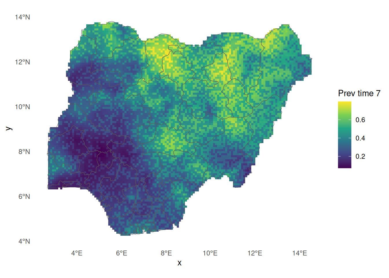
14. Predict spatio-temporal prevalence (example: time = 7)

Here we used the sum of purely spatial and purely temporal process for prediction at time 7.

Code

pred_grid$time <- 7

pred_st <- predict(
fit_st_binom,
newdata = pred_grid,
formula = ~ plogis(Intercept + beta_elev + beta_ndvi + beta_urban +
time + field),
n.samples = 500
)

Map for 2020:

Code

pred_st_r <- st_rasterize(pred_st["mean"], dx=10000, dy=10000)

ggplot() +
  geom_stars(data = pred_st_r, na.rm = TRUE) +
  scale_fill_viridis_c(name="Prev time 7", na.value = NA) +
  geom_sf(data=nga_admin1, fill=NA) +
  theme_minimal() +
  theme(
    panel.background = element_rect(fill = "white", colour = NA),
    plot.background  = element_rect(fill = "white", colour = NA),
    panel.grid       = element_blank()
  )

End of Day 1

By the end of today participants can:

Fit spatial binomial and Poisson models
Build meshes and PC priors
Predict over a grid
Generate exceedance probability maps
Fit basic spatio-temporal models using SPDE + RW1