Day 3 – Hybrid Machine Learning + Geostatistics

Author

Olatunji Johnson

Overview

Today we combine:

  • Machine learning models (e.g., Random Forest, XGBoost)
  • Spatial residual modelling via SPDE + inlabru
  • Hybrid prediction pipelines for malaria prevalence

The goal:
Use ML to model complex covariate effects, and INLA/SPDE to model spatial dependence in the residuals.

Learning objectives

By the end of Day 3 you should be able to:

  • Fit a baseline geostatistical prevalence model with SPDE/inlabru
  • Fit an ML model for the systematic component (covariate-driven signal)
  • Diagnose spatial autocorrelation in residuals
  • Fit a spatial residual model to ML residuals
  • Combine ML + spatial residuals into a single hybrid prediction surface
  • Map predictions and uncertainty clipped to Nigeria

Load Day 3 dataset

Code
library(tidyverse)
library(sf)
library(ggplot2)

hybrid_ml_geo <- read_csv("data/hybrid_ml_geostatistical_data.csv")
head(hybrid_ml_geo)
# A tibble: 6 × 11
     id   utm_x    utm_y n_tested n_pos prevalence_true ml_signal_true
  <dbl>   <dbl>    <dbl>    <dbl> <dbl>           <dbl>          <dbl>
1     1 279090.  838870.       63     0        0.00167           -5.04
2     2  57751.  672968.      125     0        0.000452          -6.60
3     3 160759. 1365476.      139     0        0.00694           -3.80
4     4 949111. 1230481.      126     0        0.000334          -7.10
5     5 434005.  682490.       97     0        0.00205           -5.51
6     6 -91406.  925776.      122     3        0.00767           -3.16
# ℹ 4 more variables: S_residual_true <dbl>, elevation <dbl>, ndvi <dbl>,
#   urban <dbl>

Convert to sf

Code
hybrid_sf <- hybrid_ml_geo |>
st_as_sf(coords = c("utm_x","utm_y"), crs = 32632)

Part 1 — Baseline: purely geostatistical model

Model \[Y_i | p_i = \text{Binomial}(N_i,p_i), \quad \text{logit}(p_i) = \beta_0 + \beta^\top x_i + S(s_i).\] This is the “standard” MBG model:

  • interpretable
  • principled uncertainty
  • but limited if covariate effects are highly nonlinear

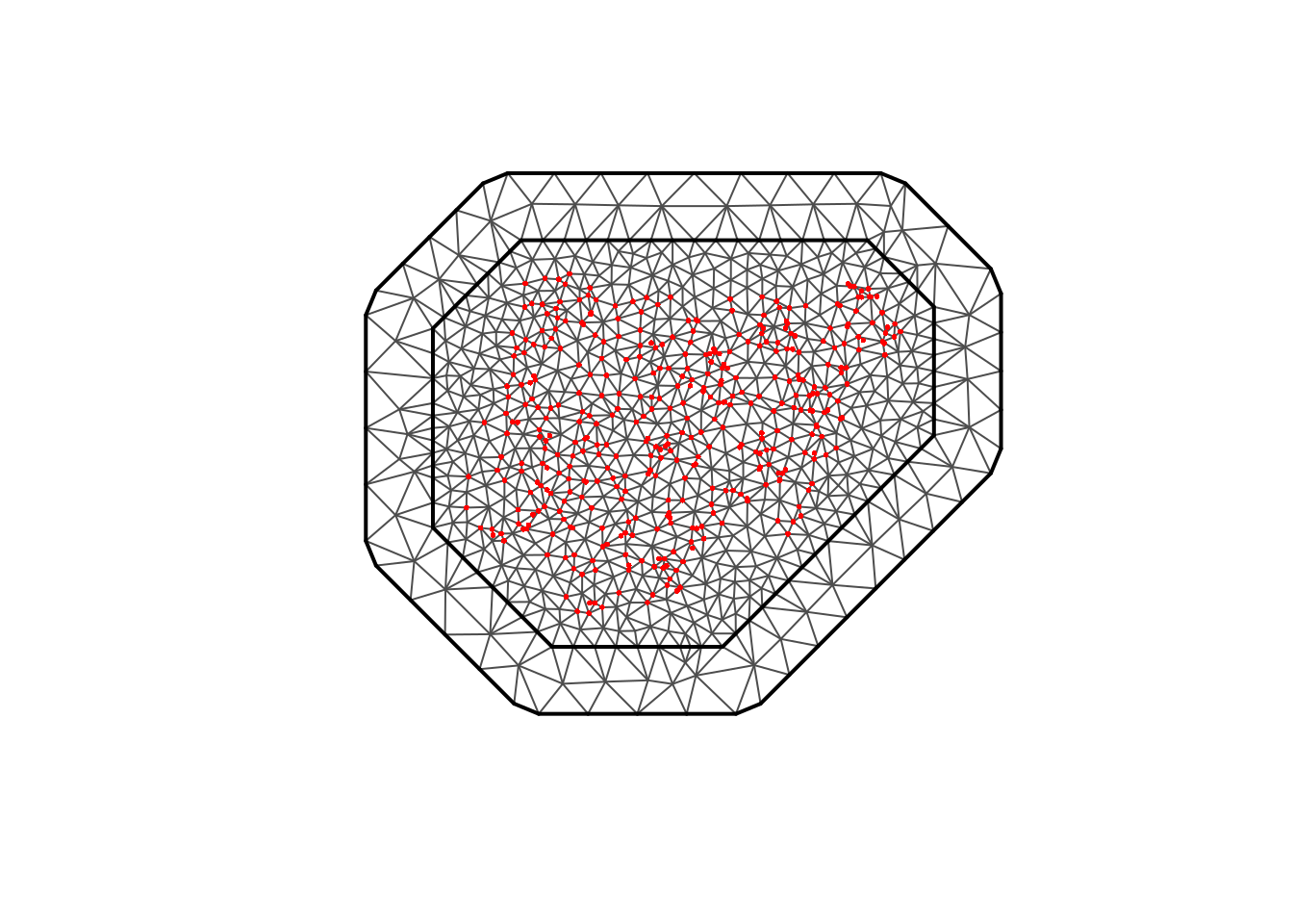
Build SPDE mesh

Code
library(INLA)
library(inlabru)

mesh <- inla.mesh.2d(
loc = st_coordinates(hybrid_sf),
max.edge = c(80000, 250000),
cutoff   = 20000,
offset   = c(100000, 200000)
)

plot(mesh)
points(st_coordinates(hybrid_sf), pch = 16, cex = 0.4, col = "red")

Define SPDE prior (PC priors)

Code
spde <- inla.spde2.pcmatern(
mesh = mesh,
prior.range = c(300000, 0.5),
prior.sigma = c(1, 0.5)
)

Fit baseline geostatistical model

Code
hybrid_dat <- hybrid_sf |>
mutate(y = n_pos, n = n_tested)

cmp_base <- y ~ 1 + elevation + ndvi + urban +
field(geometry, model = spde)

fit_base <- bru(
components = cmp_base,
family = "binomial",
data = hybrid_dat,
Ntrials = hybrid_dat$n
)

summary(fit_base)
inlabru version: 2.13.0.9024 
INLA version: 25.12.02 
Latent components:
elevation: main = linear(elevation)
ndvi: main = linear(ndvi)
urban: main = linear(urban)
field: main = spde(geometry)
Intercept: main = linear(1)
Observation models:
  Model tag: <No tag>
    Family: 'binomial'
    Data class: 'sf', 'tbl_df', 'tbl', 'data.frame'
    Response class: 'numeric'
    Predictor: y ~ elevation + ndvi + urban + field + Intercept
    Additive/Linear/Rowwise: TRUE/TRUE/TRUE
    Used components: effect[elevation, ndvi, urban, field, Intercept], latent[] 
Time used:
    Pre = 0.99, Running = 2.36, Post = 0.405, Total = 3.75 
Fixed effects:
            mean    sd 0.025quant 0.5quant 0.975quant   mode kld
elevation -0.025 0.002     -0.029   -0.025     -0.021 -0.025   0
ndvi       1.470 0.510      0.451    1.474      2.464  1.473   0
urban      0.983 0.132      0.724    0.983      1.243  0.983   0
Intercept  0.706 0.595     -0.449    0.701      1.891  0.701   0

Random effects:
  Name    Model
    field SPDE2 model

Model hyperparameters:
                    mean       sd 0.025quant 0.5quant 0.975quant    mode
Range for field 8.07e+04 4.72e+04   2.50e+04 6.94e+04   2.04e+05 5.2e+04
Stdev for field 5.88e-01 1.37e-01   3.59e-01 5.74e-01   8.94e-01 5.5e-01

Marginal log-Likelihood:  -430.18 
 is computed 
Posterior summaries for the linear predictor and the fitted values are computed
(Posterior marginals needs also 'control.compute=list(return.marginals.predictor=TRUE)')

Part 2 — ML systematic component (explain covariates flexibly)

Why ML?

Classical linear terms assume:

\[\eta(s) = \beta_0 + \beta_1 \text{ndvi} + \beta_2 \text{elev} + \beta_3 \text{urban}\] But in practice:

  • nonlinear responses (e.g., risk peaks at intermediate NDVI)
  • interactions (e.g., urban × elevation)

ML models are good at learning this.

Target for ML

We want ML to model the systematic component. There are two common choices: A) ML on prevalence and B) ML on the transformed prevalence (empirical logit transformation). We will use B in this tutorial. There are many other transformations that can be considered. Hence, we can create a pseudo-response: \[\tilde{\eta}_i = \text{log}\left(\frac{y_i + 0.5}{n_i -y_i +0.5}\right)\]

Then we will use ML to predict \(\tilde{\eta}_i\)

Create ML training response (logit-prevalence)

Code
ml_df <- hybrid_ml_geo |>
mutate(
prev_obs = n_pos / n_tested,
eta_obs = log((n_pos + 0.5) / (n_tested - n_pos + 0.5))  
)

summary(ml_df$eta_obs)
   Min. 1st Qu.  Median    Mean 3rd Qu.    Max. 
 -5.994  -5.541  -4.977  -4.845  -4.316  -2.174 

Train/test split

Code
set.seed(123)
idx <- sample(seq_len(nrow(ml_df)), size = floor(0.8 * nrow(ml_df)))

train_df <- ml_df[idx, ]
test_df  <- ml_df[-idx, ]

ML model 1: Random Forest (quick baseline)

Code
library(ranger)

rf_fit <- ranger(
eta_obs ~ elevation + ndvi + urban,
data = train_df,
num.trees = 500,
importance = "impurity"
)

rf_fit
Ranger result

Call:
 ranger(eta_obs ~ elevation + ndvi + urban, data = train_df, num.trees = 500,      importance = "impurity") 

Type:                             Regression 
Number of trees:                  500 
Sample size:                      320 
Number of independent variables:  3 
Mtry:                             1 
Target node size:                 5 
Variable importance mode:         impurity 
Splitrule:                        variance 
OOB prediction error (MSE):       0.4730291 
R squared (OOB):                  0.3906921 

Evaluate RF performance

Code
test_pred_rf <- predict(rf_fit, data = test_df)$predictions

rmse_rf <- sqrt(mean((test_pred_rf - test_df$eta_obs)^2))
rmse_rf
[1] 0.7333414

Variable importance (RF)

Code
sort(rf_fit$variable.importance, decreasing = TRUE)
elevation      ndvi     urban 
 83.66540  34.37766  15.95882 

ML model 2: XGBoost (often stronger)

Code
library(xgboost)

X_train <- model.matrix(~ elevation + ndvi + urban, train_df)[,-1]
X_test  <- model.matrix(~ elevation + ndvi + urban, test_df)[,-1]

dtrain <- xgb.DMatrix(data = X_train, label = train_df$eta_obs)
dtest  <- xgb.DMatrix(data = X_test,  label = test_df$eta_obs)

params <- list(
  objective = "reg:squarederror",
  eval_metric = "rmse",
  eta = 0.05,
  max_depth = 4,
  subsample = 0.8,
  colsample_bytree = 0.9
)

xgb_fit <- xgb.train(
  params = params,
  data = dtrain,
  nrounds = 400,
  evals = list(train = dtrain, test = dtest),
  verbose = 0
)

test_pred_xgb <- predict(xgb_fit, dtest)
rmse_xgb <- sqrt(mean((test_pred_xgb - test_df$eta_obs)^2))
rmse_xgb
[1] 0.8283068

Which ML model should we use?

Pick the model with:

  • better predictive performance (RMSE)
  • stable behaviour
  • interpretability

For the hybrid pipeline, either is fine. We proceed with RF, but XGBoost works similarly.

Part 3 — Spatial residual modelling of ML residuals

The key diagnostic question

After ML, compute residuals: \[r_i = \tilde{\eta}_i - \hat{m}(x_i),\] where \(\hat{m}\) is the ML prediction. If \(r_i\) shows evidence of spatial correlation, then ML has a missing spatial structure. We then model: \[r_i = S(s_i) + \epsilon_i.\]

Compute ML residuals

Code
# ml_pred_all <- predict(
# xgb_fit,
# xgb.DMatrix(model.matrix(~ elevation + ndvi + urban, ml_df)[,-1])
# )
# 
# ml_df <- ml_df |>
# mutate(
# eta_ml = ml_pred_all,
# resid_ml = eta_obs - eta_ml
# )
# 
# summary(ml_df$resid_ml)


ml_pred_all <- predict(rf_fit, data = ml_df)$predictions

ml_df <- ml_df |>
  mutate(
    eta_ml = ml_pred_all,
    resid_ml = eta_obs - eta_ml
  )

summary(ml_df$resid_ml)
    Min.  1st Qu.   Median     Mean  3rd Qu.     Max. 
-1.52115 -0.46093 -0.01799  0.01231  0.47075  1.51275 

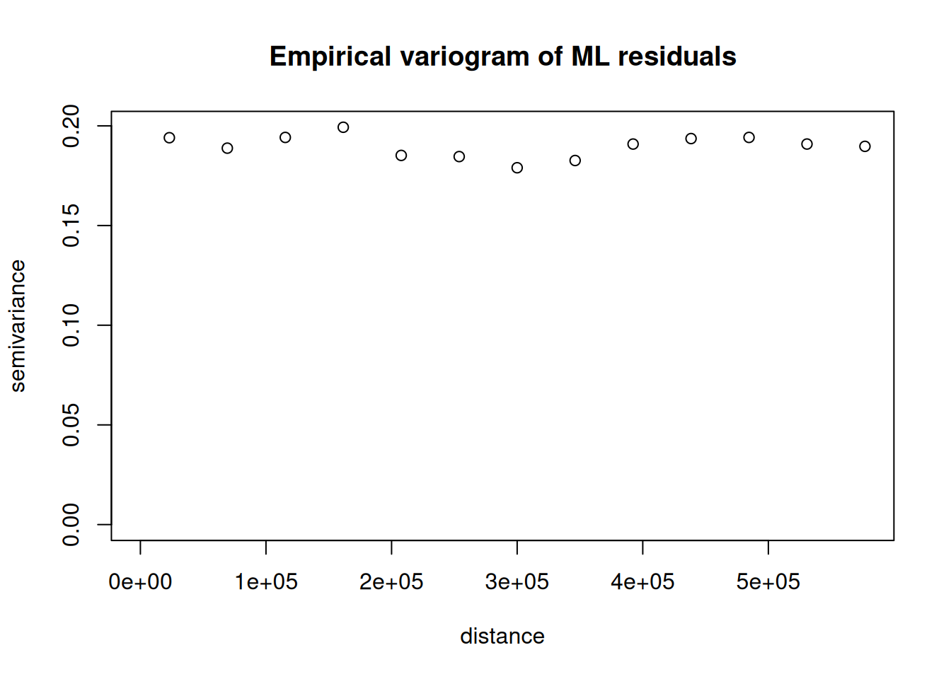
Variogram of the residual

Code
library(geoR)

coords <- ml_df[, c("utm_x","utm_y")]
geodata <- as.geodata(
cbind(coords, ml_df$resid_ml),
coords.col = 1:2,
data.col = 3
)

v <- variog(geodata, max.dist = 600000)
variog: computing omnidirectional variogram
Code
plot(v, main = "Empirical variogram of ML residuals")

Code
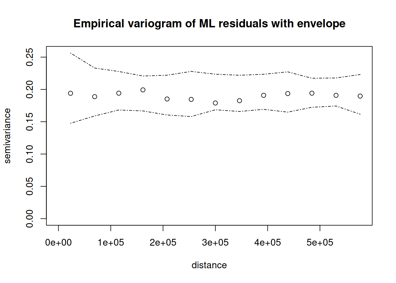
vari.mc <- variog.mc.env(geodata, obj.variog=v, nsim=1000)
variog.env: generating 1000 simulations by permutating data values
variog.env: computing the empirical variogram for the 1000 simulations
variog.env: computing the envelops
Code
plot(v, envelope.obj=vari.mc, main = "Empirical variogram of ML residuals with envelope")

Fit spatial model to residuals (Gaussian likelihood)

Residuals are approximately continuous, so we use:

\[r_i \sim \text{N}(\mu_i, \sigma_\epsilon), \quad \mu_i = S(s_i)\]

This gives a clean two-stage hybrid approach.

Build sf + mesh for residual model

Code
resid_sf <- ml_df |>
st_as_sf(coords = c("utm_x","utm_y"), crs = 32632)

mesh_r <- inla.mesh.2d(
loc = st_coordinates(resid_sf),
max.edge = c(80000, 250000),
cutoff   = 20000,
offset   = c(100000, 200000)
)

spde_r <- inla.spde2.pcmatern(
mesh = mesh_r,
prior.range = c(300000, 0.5),
prior.sigma = c(1, 0.5)
)

Fit spatial residual model in inlabru

Code
cmp_resid <- resid_ml ~ 1 +
resid_field(geometry, model = spde_r)

fit_resid <- bru(
components = cmp_resid,
family = "gaussian",
data = resid_sf
)

summary(fit_resid)
inlabru version: 2.13.0.9024 
INLA version: 25.12.02 
Latent components:
resid_field: main = spde(geometry)
Intercept: main = linear(1)
Observation models:
  Model tag: <No tag>
    Family: 'gaussian'
    Data class: 'sf', 'tbl_df', 'tbl', 'data.frame'
    Response class: 'numeric'
    Predictor: resid_ml ~ resid_field + Intercept
    Additive/Linear/Rowwise: TRUE/TRUE/TRUE
    Used components: effect[resid_field, Intercept], latent[] 
Time used:
    Pre = 1.08, Running = 1.53, Post = 0.154, Total = 2.76 
Fixed effects:
            mean    sd 0.025quant 0.5quant 0.975quant   mode kld
Intercept -0.001 0.033     -0.067   -0.001      0.068 -0.001   0

Random effects:
  Name    Model
    resid_field SPDE2 model

Model hyperparameters:
                                            mean       sd 0.025quant 0.5quant
Precision for the Gaussian observations 5.33e+00 4.36e-01   4.51e+00 5.32e+00
Range for resid_field                   3.21e+05 4.54e+05   2.97e+04 1.87e+05
Stdev for resid_field                   8.40e-02 4.40e-02   2.40e-02 7.60e-02
                                        0.975quant     mode
Precision for the Gaussian observations   6.22e+00 5.31e+00
Range for resid_field                     1.45e+06 7.46e+04
Stdev for resid_field                     1.92e-01 5.80e-02

Marginal log-Likelihood:  -260.22 
 is computed 
Posterior summaries for the linear predictor and the fitted values are computed
(Posterior marginals needs also 'control.compute=list(return.marginals.predictor=TRUE)')

Part 4 — Hybrid predictions: ML + spatial residual surface

Hybrid predictor on logit scale

For any location \(s\):

\[\hat{\eta}_\text{hyb} (s) = \hat{m}(x(s)) + \hat{S}(s)\] Then the prevalence becomes \[\hat{p}_\text{hyb} (s) = \text{logit}^{-1} (\hat{\eta}_\text{hyb} (s))\]

Nigeria boundaries and prediction grid

Code
nga_admin1 <- st_read("data/nga_shapefile.shp") 
Reading layer `nga_shapefile' from data source 
  `/home/olatunji-johnson/Documents/Manchester Job/Teaching/Courses/Nigeria_2026/rcode/FUTA/data/nga_shapefile.shp' 
  using driver `ESRI Shapefile'
Simple feature collection with 37 features and 121 fields
Geometry type: MULTIPOLYGON
Dimension:     XY
Bounding box:  xmin: -198992.3 ymin: 472813 xmax: 1117766 ymax: 1537228
Projected CRS: WGS 84 / UTM zone 32N
Code
nga_poly <- st_union(nga_admin1)

pred_grid_sf <- read_csv("data/prediction_grid_utm.csv") |>
st_as_sf(coords = c("utm_x","utm_y"), crs = 32632)

# clip grid to Nigeria
# 
# inside <- st_within(pred_grid_sf, nga_poly, sparse = FALSE)[,1]
# pred_grid_sf <- pred_grid_sf[inside, ]

Step 1: ML predictions on the grid

Code
# Xg <- model.matrix(~ elevation + ndvi + urban, st_drop_geometry(pred_grid_sf))[,-1]
# pred_grid_sf$eta_ml <- predict(xgb_fit, xgb.DMatrix(Xg))

pred_grid_sf$eta_ml <- predict(rf_fit, data = st_drop_geometry(pred_grid_sf))$predictions

Step 2: Spatial residual predictions on the grid

Code
pred_resid <- predict(
fit_resid,
newdata = pred_grid_sf,
formula = ~ resid_field,
n.samples = 200
)

pred_grid_sf$resid_mean <- pred_resid$mean

Combine into hybrid prevalence

Code
pred_grid_sf$eta_hybrid <- pred_grid_sf$eta_ml + pred_grid_sf$resid_mean
pred_grid_sf$prev_hybrid <- plogis(pred_grid_sf$eta_hybrid)

summary(pred_grid_sf$prev_hybrid)
    Min.  1st Qu.   Median     Mean  3rd Qu.     Max. 
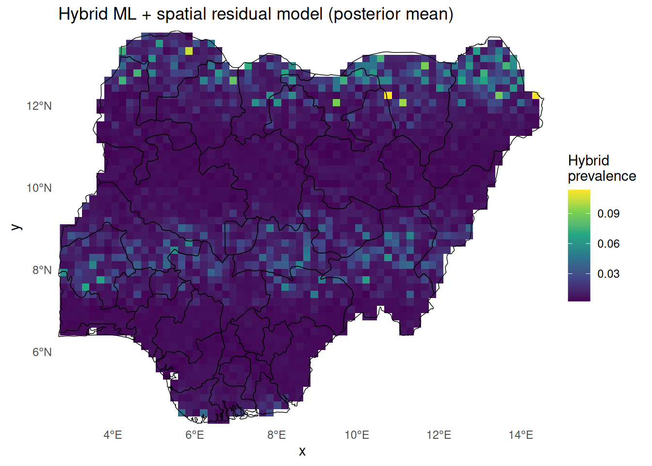
0.002208 0.004939 0.006543 0.010814 0.010921 0.141775 

Rasterise + map (clipped to Nigeria)

Code
library(stars)

pred_rast <- st_rasterize(pred_grid_sf["prev_hybrid"], dx = 20000, dy = 20000)
pred_rast_ng <- pred_rast[nga_poly]

ggplot() +
geom_stars(data = pred_rast_ng, na.rm = TRUE) +
geom_sf(data = nga_admin1, fill = NA, colour = "black", linewidth = 0.25) +
coord_sf(expand = FALSE) +
scale_fill_viridis_c(name = "Hybrid\nprevalence", na.value = NA) +
theme_minimal() +
theme(panel.grid = element_blank(),
panel.background = element_rect(fill = "white", colour = NA),
plot.background  = element_rect(fill = "white", colour = NA)) +
labs(title = "Hybrid ML + spatial residual model (posterior mean)")

Where does uncertainty come from?

Hybrid model uncertainty includes:

  1. ML uncertainty (often ignored unless using Bayesian ML / ensembles)
  2. Spatial residual uncertainty (captured via INLA posterior)
  3. Observation noise and binomial sampling noise

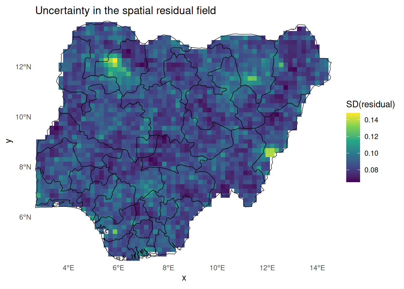
In this workshop we quantify (2).

Map posterior SD of spatial residual field

Code
pred_grid_sf$resid_sd <- pred_resid$sd

sd_rast <- st_rasterize(pred_grid_sf["resid_sd"], dx = 20000, dy = 20000)[nga_poly]

ggplot() +
geom_stars(data = sd_rast, na.rm = TRUE) +
geom_sf(data = nga_admin1, fill = NA, colour = "black", linewidth = 0.25) +
coord_sf(expand = FALSE) +
scale_fill_viridis_c(name = "SD(residual)", na.value = NA) +
theme_minimal() +
theme(panel.grid = element_blank(),
panel.background = element_rect(fill = "white", colour = NA),
plot.background  = element_rect(fill = "white", colour = NA)) +
labs(title = "Uncertainty in the spatial residual field")

Part 6 — Comparison: baseline geostatistical vs hybrid

Why compare?

Baseline model already uses a spatial field + covariates. Hybrid model changes the systematic part by using ML.

We compare:

  • prediction accuracy (held-out sites)
  • residual spatial structure
  • plausibility of surfaces

Compare predictive accuracy on held-out data

Code
# baseline fitted values (posterior mean)

base_pred <- predict(
fit_base,
newdata = hybrid_dat,
formula = ~ plogis(Intercept + elevation + ndvi + urban + field)
)$mean

# hybrid fitted values

hyb_pred <- plogis(ml_df$eta_ml + predict(fit_resid, newdata = resid_sf, formula = ~ resid_field)$mean)

obs_prev <- hybrid_ml_geo$n_pos / hybrid_ml_geo$n_tested

rmse_base <- sqrt(mean((base_pred - obs_prev)^2))
rmse_hyb  <- sqrt(mean((hyb_pred - obs_prev)^2))

c(rmse_base = rmse_base, rmse_hyb = rmse_hyb)
  rmse_base    rmse_hyb 
0.006897612 0.006705097