Day 2 – Joint modelling and Non-stationary processes

Author

Olatunji Johnson

Overview

Today we will cover two key advanced topics in spatial modelling:

Joint modelling of multiple malaria processes
- Shared spatial fields
- Process-specific fields
- Multiple outcomes (e.g., children vs pregnant women)
- Multiple likelihoods (Binomial + Poisson)
Non-stationary spatial processes
- Region-varying smoothness
- Covariate-driven nonstationarity
- Combining multiple spatial SPDEs

1. Load Day 2 datasets

Code

library(tidyverse)
library(INLA)
library(inlabru)
library(ggplot2)
library(sf)
library(stars)
library(geoR)

joint_malaria <- read_csv("data/joint_malaria_processes.csv")
nonstat_malaria <- read_csv("data/nonstationary_malaria_data.csv")

nga_admin1 <- st_read("data/nga_shapefile.shp")

Reading layer `nga_shapefile' from data source 
  `/home/olatunji-johnson/Documents/Manchester Job/Teaching/Courses/Nigeria_2026/rcode/FUTA/data/nga_shapefile.shp' 
  using driver `ESRI Shapefile'
Simple feature collection with 37 features and 121 fields
Geometry type: MULTIPOLYGON
Dimension:     XY
Bounding box:  xmin: -198992.3 ymin: 472813 xmax: 1117766 ymax: 1537228
Projected CRS: WGS 84 / UTM zone 32N

Code

head(joint_malaria)

# A tibble: 6 × 12
     id group    utm_x  utm_y n_tested n_pos prevalence_true S_shared S_specific
  <dbl> <chr>    <dbl>  <dbl>    <dbl> <dbl>           <dbl>    <dbl>      <dbl>
1     1 child… 249196. 7.37e5      148    48           0.281   0.297      -0.409
2     2 child… 703934. 9.57e5      107    35           0.337  -0.0736      0.415
3     3 child… -90558. 9.32e5      139    66           0.416   0.680      -0.145
4     4 child… 252087. 1.11e6      138    55           0.369  -0.147       0.277
5     5 child… 685078. 1.34e6      183    47           0.219  -0.192      -0.281
6     6 child… 422901. 5.12e5      131    63           0.501   0.589       0.166
# ℹ 3 more variables: elevation <dbl>, ndvi <dbl>, urban <dbl>

2. Convert to sf for mapping

We need an sf layer to overlay boundaries, plot points, and feed coordinates into SPDE meshes.

Code

joint_malaria_sf <- joint_malaria %>%
  st_as_sf(coords = c("utm_x", "utm_y"), crs = 32632)
nonstat_malaria_sf <- nonstat_malaria %>%
  st_as_sf(coords = c("utm_x", "utm_y"), crs = 32632)

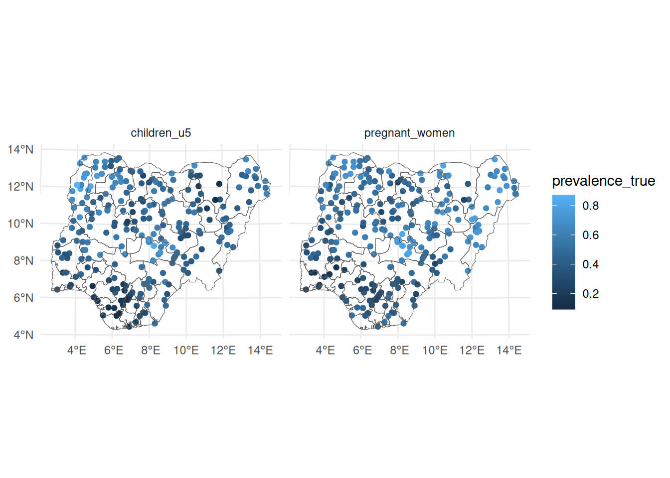
3. Quick visualisation

Code

ggplot() +
geom_sf(data = joint_malaria_sf, aes(colour = prevalence_true)) +
facet_wrap(~group) +
geom_sf(data = nga_admin1, fill = NA) +
geom_point() +
theme_minimal()

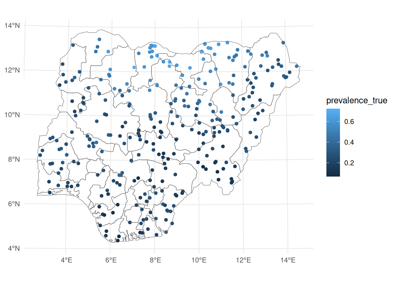
Quick visualisation (non-stationary dataset)

Code

ggplot() +
geom_sf(data = nonstat_malaria_sf, aes(colour = prevalence_true)) +
geom_sf(data = nga_admin1, fill = NA) +
geom_point() +
theme_minimal()

============================================================

Part 1A — Joint modelling (shared + group-specific fields)

============================================================

4. Create a single stacked dataset

We will model both groups jointly with: - one shared spatial field - one group-specific spatial field (replicated by group)

Code

joint_dat <- joint_malaria_sf |>
mutate(
group = factor(group),
y = n_pos,
n = n_tested
)

levels(joint_dat$group)

[1] "children_u5"    "pregnant_women"

5. Build SPDE mesh

Code

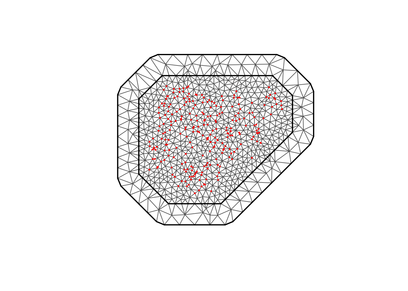
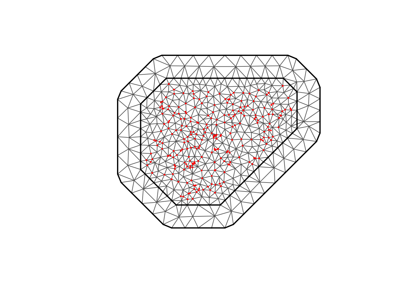
locs_joint <- joint_malaria_sf

mesh_joint <- inla.mesh.2d(
loc = st_coordinates(locs_joint),
max.edge = c(80000, 250000),   # tune for smoothness vs speed
cutoff = 20000,                # remove very close points
offset = c(100000, 200000)
)

plot(mesh_joint)
points(st_coordinates(locs_joint), pch = 16, cex = 0.4, col= "red")

6. Define SPDEs (shared + group-specific)

spde_shared: one latent field for all data
spde_group: replicated field with one replicate per group

Code

spde_shared <- inla.spde2.pcmatern(
mesh = mesh_joint,
prior.range = c(300000, 0.5),   # P(range < 300km) = 0.5
prior.sigma = c(1, 0.5)         # P(sigma > 1) = 0.5
)

spde_group <- inla.spde2.pcmatern(
mesh = mesh_joint,
prior.range = c(200000, 0.5),
prior.sigma = c(1, 0.5)
)

7. Fit joint model in inlabru

Model:

Binomial likelihood for counts
Fixed effects (elevation, ndvi, urban)
field_shared() applies to all
field_group() replicated by group

Code

cmp_joint <- y ~
1 +
elevation + ndvi + urban +
field_shared(geometry, model = spde_shared) +
field_group(geometry, model = spde_group, replicate = group)

fit_joint <- bru(
components = cmp_joint,
family = "binomial",
data = joint_dat,
Ntrials = joint_dat$n,
options = list(control.compute = list(dic = TRUE, waic = TRUE))
)

summary(fit_joint)

inlabru version: 2.13.0.9024 
INLA version: 25.12.02 
Latent components:
elevation: main = linear(elevation)
ndvi: main = linear(ndvi)
urban: main = linear(urban)
field_shared: main = spde(geometry)
field_group: main = spde(geometry), replicate = iid(group)
Intercept: main = linear(1)
Observation models:
  Model tag: <No tag>
    Family: 'binomial'
    Data class: 'sf', 'tbl_df', 'tbl', 'data.frame'
    Response class: 'numeric'
    Predictor: y ~ elevation + ndvi + urban + field_shared + field_group + Intercept
    Additive/Linear/Rowwise: TRUE/TRUE/TRUE
    Used components: effect[elevation, ndvi, urban, field_shared, field_group, Intercept], latent[] 
Time used:
    Pre = 1.06, Running = 10.3, Post = 0.419, Total = 11.7 
Fixed effects:
            mean    sd 0.025quant 0.5quant 0.975quant   mode kld
elevation -0.002 0.001     -0.003   -0.002      0.000 -0.002   0
ndvi       1.650 0.530      0.617    1.645      2.713  1.646   0
urban      0.350 0.041      0.269    0.350      0.430  0.350   0
Intercept -0.396 0.360     -1.113   -0.393      0.304 -0.393   0

Random effects:
  Name    Model
    field_shared SPDE2 model
   field_group SPDE2 model

Model hyperparameters:
                           mean       sd 0.025quant 0.5quant 0.975quant
Range for field_shared 5.32e+04 1.62e+04   2.81e+04 5.09e+04   9.12e+04
Stdev for field_shared 3.47e-01 3.60e-02   2.81e-01 3.46e-01   4.23e-01
Range for field_group  3.41e+05 6.04e+04   2.42e+05 3.34e+05   4.78e+05
Stdev for field_group  5.37e-01 6.50e-02   4.24e-01 5.32e-01   6.78e-01
                           mode
Range for field_shared 4.68e+04
Stdev for field_shared 3.43e-01
Range for field_group  3.19e+05
Stdev for field_group  5.19e-01

Deviance Information Criterion (DIC) ...............: 3183.49
Deviance Information Criterion (DIC, saturated) ....: 835.78
Effective number of parameters .....................: 292.18

Watanabe-Akaike information criterion (WAIC) ...: 3175.37
Effective number of parameters .................: 214.05

Marginal log-Likelihood:  -1807.95 
 is computed 
Posterior summaries for the linear predictor and the fitted values are computed
(Posterior marginals needs also 'control.compute=list(return.marginals.predictor=TRUE)')

8. Prediction grid inside Nigeria (UTM)

Code

# make_grid_utm <- function(polygon_utm, dx = 20000) {
# bb <- st_bbox(polygon_utm)
# xs <- seq(bb["xmin"], bb["xmax"], by = dx)
# ys <- seq(bb["ymin"], bb["ymax"], by = dx)
# grid <- expand.grid(utm_x = xs, utm_y = ys)
# pts  <- st_as_sf(grid, coords = c("utm_x", "utm_y"), crs = st_crs(polygon_utm))
# inside <- st_within(pts, polygon_utm, sparse = FALSE)[, 1]
# grid[inside, ]
# }
# 
# pred_grid_joint <- make_grid_utm(nga_poly %>% st_transform(32632), dx = 100000) |>
# mutate(
# # For teaching: use simple smooth-ish covariates (replace with real rasters later)
# elevation = 250 + 80 * scale(utm_y)[,1] + rnorm(n(), sd = 15),
# ndvi      = plogis(-0.2 + 0.8 * scale(utm_y)[,1] + 0.3 * sin(scale(utm_x)[,1])),
# urban     = rbinom(n(), 1, plogis(-0.2 + 0.3 * scale(utm_x)[,1]))
# )

pred_grid_joint <- read_csv("data/prediction_grid_utm.csv") %>% 
tidyr::expand_grid(group = levels(joint_dat$group)) %>%
st_as_sf(coords=c("utm_x","utm_y"), crs=32632)
head(pred_grid_joint)

Simple feature collection with 6 features and 6 fields
Geometry type: POINT
Dimension:     XY
Bounding box:  xmin: 172259.6 ymin: 478133.5 xmax: 185657.6 ymax: 478184.5
Projected CRS: WGS 84 / UTM zone 32N
# A tibble: 6 × 7
    lon   lat elevation   ndvi urban group                     geometry
  <dbl> <dbl>     <dbl>  <dbl> <dbl> <chr>                  <POINT [m]>
1  6.05  4.32      253. 0.0664     1 children_u5    (172259.6 478184.5)
2  6.05  4.32      253. 0.0664     1 pregnant_women (172259.6 478184.5)
3  6.11  4.32      244. 0.0654     1 children_u5    (178958.8 478158.8)
4  6.11  4.32      244. 0.0654     1 pregnant_women (178958.8 478158.8)
5  6.17  4.32      242. 0.0645     1 children_u5    (185657.6 478133.5)
6  6.17  4.32      242. 0.0645     1 pregnant_women (185657.6 478133.5)

9. Predict for each group and map

Code

pred_joint <- predict(
fit_joint,
newdata = pred_grid_joint,
formula = ~ plogis(Intercept + elevation + ndvi + urban +
field_shared + field_group),
n.samples = 200
)

pred_joint_sf <- pred_joint |>
rename(prev_mean = mean)

head(pred_joint_sf)

Simple feature collection with 6 features and 14 fields
Geometry type: POINT
Dimension:     XY
Bounding box:  xmin: 172259.6 ymin: 478133.5 xmax: 185657.6 ymax: 478184.5
Projected CRS: WGS 84 / UTM zone 32N
       lon      lat elevation       ndvi urban          group prev_mean
1 6.047644 4.320444  252.9367 0.06636150     1    children_u5 0.2454142
2 6.047644 4.320444  252.9367 0.06636150     1 pregnant_women 0.5502509
3 6.107940 4.320444  244.1864 0.06535912     1    children_u5 0.2431139
4 6.107940 4.320444  244.1864 0.06535912     1 pregnant_women 0.5562642
5 6.168235 4.320444  242.2228 0.06445763     1    children_u5 0.2392009
6 6.168235 4.320444  242.2228 0.06445763     1 pregnant_women 0.5595819
          sd    q0.025      q0.5    q0.975    median mean.mc_std_err
1 0.08483441 0.1175872 0.2320009 0.4295042 0.2320009     0.006635328
2 0.10346490 0.3383491 0.5534975 0.7451256 0.5534975     0.008062772
3 0.07796974 0.1296129 0.2322176 0.4115017 0.2322176     0.006096718
4 0.09640754 0.3675169 0.5628076 0.7359455 0.5628076     0.007501434
5 0.07206476 0.1319077 0.2296956 0.3944603 0.2296956     0.005632434
6 0.09133494 0.3860712 0.5576584 0.7322711 0.5576584     0.007085350
  sd.mc_std_err                  geometry
1   0.004501648 POINT (172259.6 478184.5)
2   0.005279958 POINT (172259.6 478184.5)
3   0.004125433 POINT (178958.8 478158.8)
4   0.004839379 POINT (178958.8 478158.8)
5   0.003794938 POINT (185657.6 478133.5)
6   0.004433520 POINT (185657.6 478133.5)

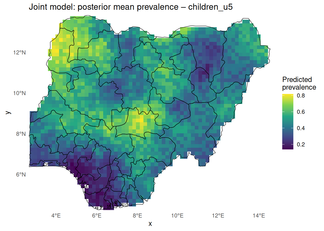
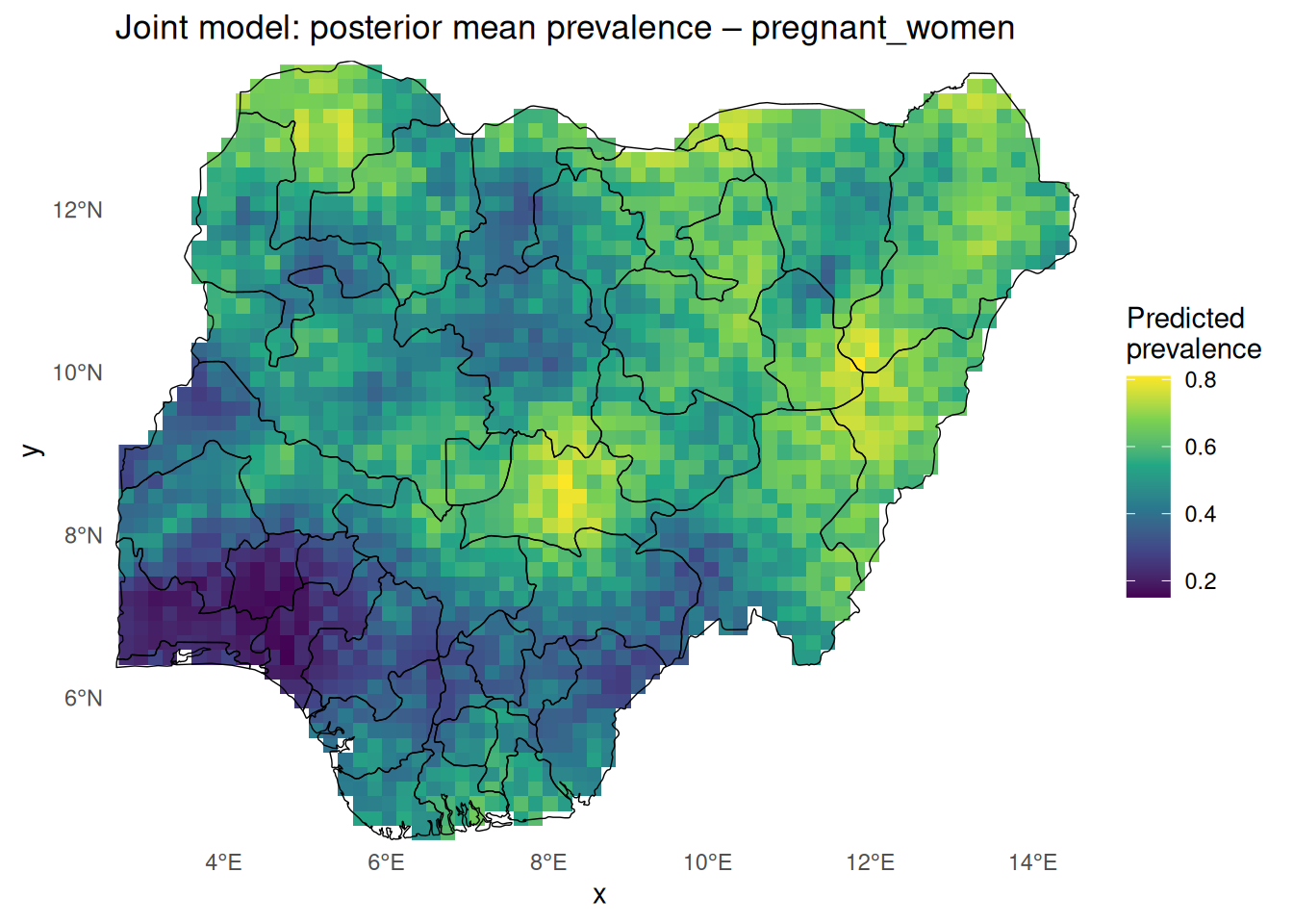
10. Raster map per group (clipped to Nigeria)

Code

pred_joint_map <- function(group_name, dx = 20000) {
dat_g <- pred_joint_sf |> filter(group == group_name)

rast <- st_rasterize(dat_g["prev_mean"], dx = dx, dy = dx)
rast_ng <- rast[st_union(nga_admin1)]

ggplot() +
geom_stars(data = rast_ng, na.rm = TRUE) +
geom_sf(data = nga_admin1, fill = NA, colour = "black", linewidth = 0.25) +
coord_sf(expand = FALSE) +
scale_fill_viridis_c(name = "Predicted\nprevalence", na.value = NA) +
theme_minimal() +
theme(panel.grid = element_blank(),
panel.background = element_rect(fill = "white", colour = NA),
plot.background  = element_rect(fill = "white", colour = NA)) +
labs(title = paste("Joint model: posterior mean prevalence –", group_name))
}

pred_joint_map("children_u5")

Code

pred_joint_map("pregnant_women")

============================================================

Part 2A — Joint modelling with multiple likelihoods (Binomial + Poisson)

============================================================

11. Prepare the two datasets and create the mesh

Here we used the binomial and poisson malaria data: - spatial_binom with n_pos, n_tested - spatial_pois with cases, population

Code

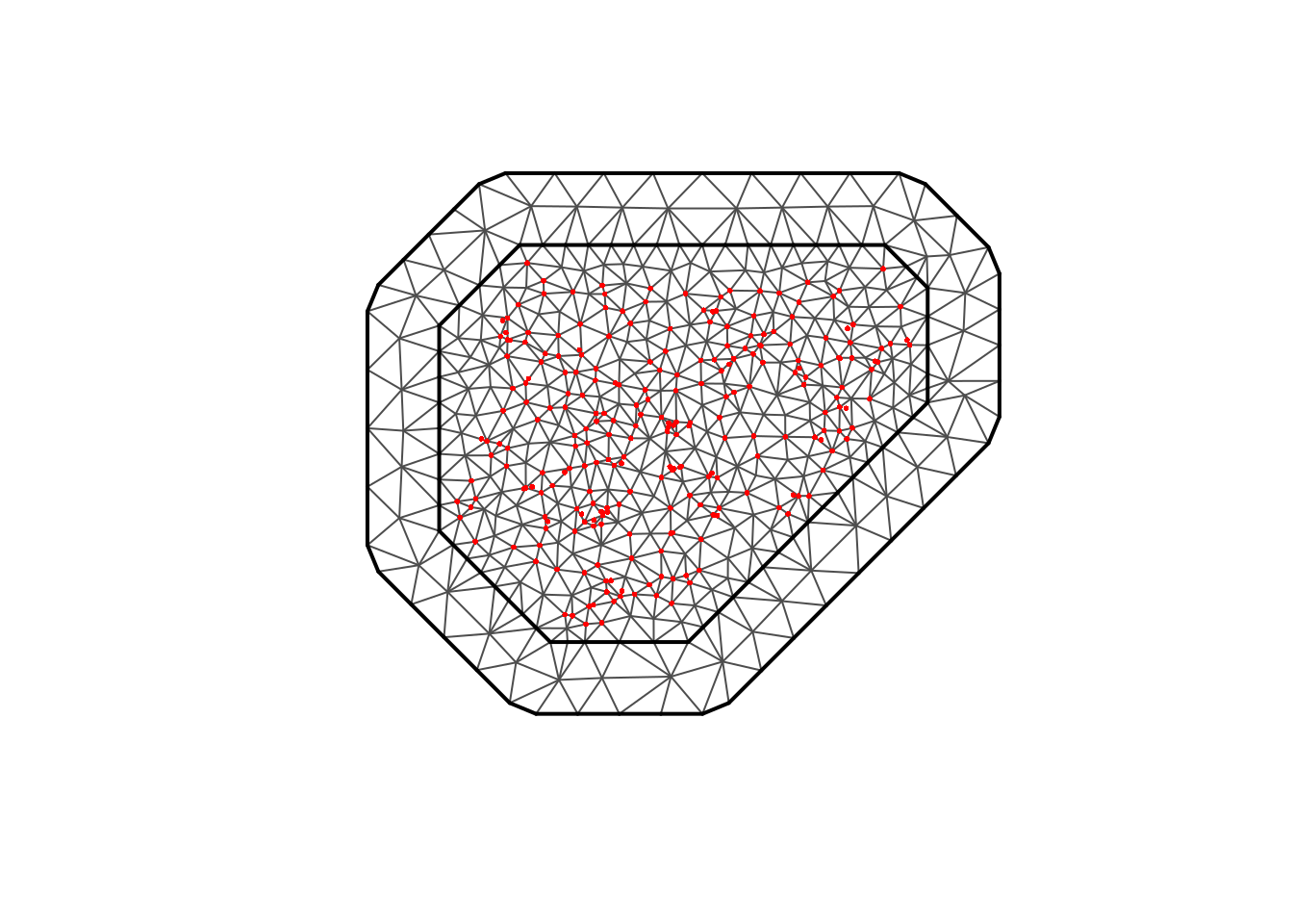
# Example: take children as binomial and pretend pregnant are poisson (toy)
binom_dat <- read_csv("data/spatial_binomial_data.csv") 
pois_dat <- read_csv("data/spatial_poisson_data.csv")

binom_sf <- st_as_sf(binom_dat, coords = c("utm_x","utm_y"), crs = 32632)
pois_sf  <- st_as_sf(pois_dat,  coords = c("utm_x","utm_y"), crs = 32632)


mesh_binom <- inla.mesh.2d(
loc = st_coordinates(binom_sf),
max.edge = c(100000, 200000), # inner and outer triangle sizes
cutoff = 20000,  # merge points closer than 20km
offset = c(50000, 200000)  # extend mesh beyond convex hull
)

plot(mesh_binom)
points(st_coordinates(binom_sf), col="red", pch=16, cex = 0.4)

Code

####
mesh_pois <- inla.mesh.2d(
loc = st_coordinates(binom_sf),
max.edge = c(100000, 200000), # inner and outer triangle sizes
cutoff = 20000,  # merge points closer than 20km
offset = c(50000, 200000)  # extend mesh beyond convex hull
)

plot(mesh_pois)
points(st_coordinates(binom_sf), col="red", pch=16, cex = 0.4)

Code

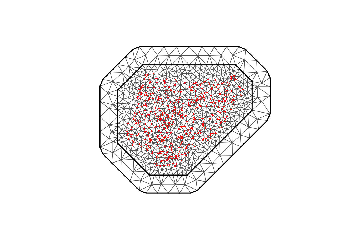
# Mesh on all locations
all_coords <- rbind(st_coordinates(binom_sf), st_coordinates(pois_sf))

mesh_joint <- inla.mesh.2d(
  loc = all_coords,
  max.edge = c(80000, 250000),
  cutoff   = 20000,
  offset   = c(100000, 200000)
)

plot(mesh_joint); points(all_coords, pch = 16, cex = 0.4, col="red")

12. Shared + likelihood-specific spatial fields

Code

spde_shared <- inla.spde2.pcmatern(
  mesh = mesh_joint,
  prior.range = c(300000, 0.5),
  prior.sigma = c(1, 0.5)
)

spde_binom <- inla.spde2.pcmatern(
  mesh = mesh_binom,
  prior.range = c(200000, 0.5),
  prior.sigma = c(1, 0.5)
)

spde_pois <- inla.spde2.pcmatern(
  mesh = mesh_pois,
  prior.range = c(200000, 0.5),
  prior.sigma = c(1, 0.5)
)

13. Fit a multi-likelihood model in inlabru

Key idea: use like() twice, and call bru() once.

Code

# Components: shared + outcome-specific fields
cmp <- ~
  Intercept_binom(1) + Intercept_pois(1) + 
  elevation + ndvi + urban +
  shared(geometry, copy = "binom_field", fixed = FALSE) +
  binom_field(geometry, model = spde_binom) +
  pois_field(geometry,  model = spde_pois)

# Likelihood 1: binomial prevalence
like_binom <- like(
  formula = n_pos ~ Intercept_binom + elevation + ndvi + urban +
  binom_field,
  family  = "binomial",
  data    = binom_sf,
  Ntrials = binom_sf$n_tested
)

# Likelihood 2: poisson cases with offset(log(population))
like_pois <- like(
  formula = cases ~ Intercept_pois + elevation + ndvi + urban +
  shared +
  pois_field, # + offset(log(population)),
  family  = "poisson",
  data    = pois_sf,
  E = pois_sf$population
)

fit_multi <- bru(
  components = cmp,
  like_binom,
  like_pois,
  options = list(control.compute = list(dic = TRUE, waic = TRUE))
)

summary(fit_multi)

inlabru version: 2.13.0.9024 
INLA version: 25.12.02 
Latent components:
Intercept_binom: main = linear(1)
elevation: main = linear(elevation)
ndvi: main = linear(ndvi)
urban: main = linear(urban)
binom_field: main = spde(geometry)
Intercept_pois: main = linear(1)
shared(=binom_field): main = unknown(geometry)
pois_field: main = spde(geometry)
Observation models:
  Model tag: <No tag>
    Family: 'binomial'
    Data class: 'sf', 'tbl_df', 'tbl', 'data.frame'
    Response class: 'numeric'
    Predictor: n_pos ~ Intercept_binom + elevation + ndvi + urban + binom_field
    Additive/Linear/Rowwise: TRUE/TRUE/TRUE
    Used components: effect[Intercept_binom, elevation, ndvi, urban, binom_field], latent[] 
  Model tag: <No tag>
    Family: 'poisson'
    Data class: 'sf', 'tbl_df', 'tbl', 'data.frame'
    Response class: 'numeric'
    Predictor: cases ~ Intercept_pois + elevation + ndvi + urban + shared + pois_field
    Additive/Linear/Rowwise: TRUE/TRUE/TRUE
    Used components: effect[Intercept_pois, elevation, ndvi, urban, shared, pois_field], latent[] 
Time used:
    Pre = 1.13, Running = 10.2, Post = 0.285, Total = 11.6 
Fixed effects:
                  mean    sd 0.025quant 0.5quant 0.975quant   mode kld
Intercept_binom -2.422 0.714     -3.790   -2.437     -0.957 -2.434   0
elevation       -0.002 0.001     -0.004   -0.002      0.000 -0.002   0
ndvi             1.935 1.044     -0.101    1.917      4.053  1.915   0
urban            0.556 0.045      0.468    0.556      0.646  0.556   0
Intercept_pois  -6.836 0.753     -8.463   -6.805     -5.428 -6.813   0

Random effects:
  Name    Model
    binom_field SPDE2 model
   pois_field SPDE2 model
   shared Copy

Model hyperparameters:
                           mean       sd 0.025quant  0.5quant 0.975quant
Range for binom_field  3.57e+05 8.09e+04   2.29e+05  3.46e+05   5.45e+05
Stdev for binom_field  1.40e+00 2.48e-01   9.90e-01  1.37e+00   1.96e+00
Range for pois_field   6.70e+05 2.72e+05   3.23e+05  6.13e+05   1.37e+06
Stdev for pois_field   7.08e-01 1.74e-01   4.45e-01  6.82e-01   1.12e+00
Beta for shared       -3.20e-02 7.90e-02  -1.90e-01 -3.20e-02   1.22e-01
                           mode
Range for binom_field  3.24e+05
Stdev for binom_field  1.31e+00
Range for pois_field   5.07e+05
Stdev for pois_field   6.25e-01
Beta for shared       -3.00e-02

Deviance Information Criterion (DIC) ...............: 2536.98
Deviance Information Criterion (DIC, saturated) ....: 819.91
Effective number of parameters .....................: 200.02

Watanabe-Akaike information criterion (WAIC) ...: 2562.60
Effective number of parameters .................: 173.60

Marginal log-Likelihood:  -1463.36 
 is computed 
Posterior summaries for the linear predictor and the fitted values are computed
(Posterior marginals needs also 'control.compute=list(return.marginals.predictor=TRUE)')

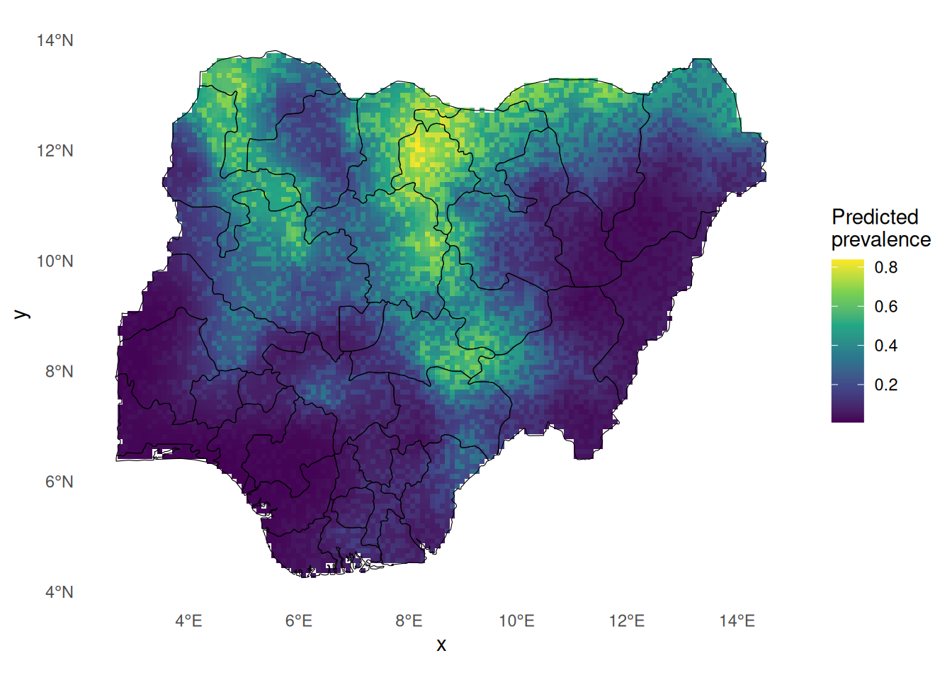
14. Predict (example: prevalence surface from the binomial part)

Code

pred_grid <- read_csv("data/prediction_grid_utm.csv") %>%
st_as_sf(coords=c("utm_x","utm_y"), crs=32632)

pred_binom_multi <- predict(
fit_multi,
newdata = pred_grid,
formula = ~ plogis(Intercept_binom + elevation + ndvi + urban + binom_field),
n.samples = 1000
)

Code

pred_binom_r <- st_rasterize(pred_binom_multi["mean"], dx=10000, dy=10000)
pred_binom_r <- pred_binom_r[st_union(nga_admin1)]
ggplot() +
  geom_stars(data=pred_binom_r, na.rm = TRUE) +
  geom_sf(data=nga_admin1, fill=NA, color = "black") +
  coord_sf() +
  scale_fill_viridis_c(name = "Predicted\nprevalence", na.value = NA) +
  theme_minimal() +
  theme(
    panel.background = element_rect(fill = "white", colour = NA),
    plot.background  = element_rect(fill = "white", colour = NA),
    panel.grid       = element_blank()
  )

============================================================

Part 1B — Non-stationary spatial process (mixture of two SPDEs)

============================================================ We’ll fit a non-stationary field using a mixture of two spatial fields:

one smooth / long-range SPDE
one rough / short-range SPDE
a spatially varying weight w(s) controlling mixture

This is a simple, teachable non-stationary construction.

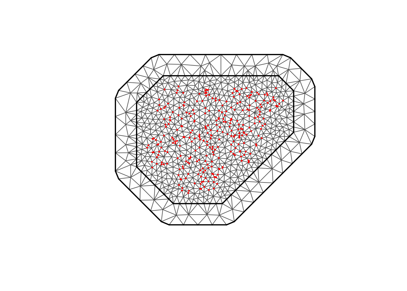
15. Prepare data and a mesh

Code

ns_dat <- nonstat_malaria |>
mutate(
y = n_pos,
n = n_tested
)

locs_ns <- nonstat_malaria_sf

mesh_ns <- inla.mesh.2d(
loc = st_coordinates(locs_ns),
max.edge = c(80000, 250000),
cutoff = 20000,
offset = c(100000, 200000)
)

plot(mesh_ns)
points(st_coordinates(locs_ns), pch = 16, cex = 0.4, col= "red")

15. Two SPDEs: smooth and rough

Code

spde_smooth <- inla.spde2.pcmatern(
mesh = mesh_ns,
prior.range = c(600000, 0.5),   # long range
prior.sigma = c(1, 0.5)
)

spde_rough <- inla.spde2.pcmatern(
mesh = mesh_ns,
prior.range = c(200000, 0.5),   # short range
prior.sigma = c(1, 0.5)
)

16. Build a spatially varying weight w(s)

Define w(s) as a simple function of northing (utm_y). (You can later replace this with a covariate surface.)

Code

# Normalised northing in [0,1]

ns_dat <- ns_dat |>
mutate(
w = (utm_y - min(utm_y)) / (max(utm_y) - min(utm_y)),
w = pmin(pmax(w, 0), 1)
) %>% st_as_sf(coords=c("utm_x","utm_y"), crs=32632)
head(ns_dat)

Simple feature collection with 6 features and 14 fields
Geometry type: POINT
Dimension:     XY
Bounding box:  xmin: -182831.5 ymin: 573963.7 xmax: 1048433 ymax: 1300816
Projected CRS: WGS 84 / UTM zone 32N
# A tibble: 6 × 15
     id n_tested n_pos prevalence_true S_nonstationary weight_north S_smooth
  <dbl>    <dbl> <dbl>           <dbl>           <dbl>        <dbl>    <dbl>
1     1      164    30           0.152         -0.793        0.168    -0.273
2     2      198    69           0.342         -0.0743       0.813     0.405
3     3      143    40           0.278         -0.0372       0.231     0.169
4     4       62    14           0.210         -0.0809       0.0903   -0.294
5     5      160    30           0.170         -0.857        0.481    -0.173
6     6      197    44           0.260         -0.0663       0.425     0.159
# ℹ 8 more variables: S_rough <dbl>, elevation <dbl>, ndvi <dbl>, urban <dbl>,
#   y <dbl>, n <dbl>, w <dbl>, geometry <POINT [m]>

17. Fit non-stationary mixture model

We model:

\[\eta = \beta_0 + \beta^\top x(s) + \omega(s) S_{smooth} + (1- \omega(s)) S_{rough}(s)\]

In inlabru we do this by multiplying the fields by covariates w and 1-w.

Code

cmp_ns <- y ~
1 + elevation + ndvi + urban +
smooth(geometry, model = spde_smooth, weights = w) +
rough(geometry, model = spde_rough,  weights = I(1 - w))

fit_ns <- bru(
components = cmp_ns,
family = "binomial",
data = ns_dat,
Ntrials = ns_dat$n,
options = list(control.compute = list(dic = TRUE, waic = TRUE))
)

summary(fit_ns)

inlabru version: 2.13.0.9024 
INLA version: 25.12.02 
Latent components:
elevation: main = linear(elevation)
ndvi: main = linear(ndvi)
urban: main = linear(urban)
smooth: main = spde(geometry), scale(w)
rough: main = spde(geometry), scale(I(1 - w))
Intercept: main = linear(1)
Observation models:
  Model tag: <No tag>
    Family: 'binomial'
    Data class: 'sf', 'tbl_df', 'tbl', 'data.frame'
    Response class: 'numeric'
    Predictor: y ~ elevation + ndvi + urban + smooth + rough + Intercept
    Additive/Linear/Rowwise: TRUE/TRUE/TRUE
    Used components: effect[elevation, ndvi, urban, smooth, rough, Intercept], latent[] 
Time used:
    Pre = 1.34, Running = 7.78, Post = 0.47, Total = 9.59 
Fixed effects:
            mean    sd 0.025quant 0.5quant 0.975quant   mode kld
elevation -0.002 0.001     -0.004   -0.002      0.000 -0.002   0
ndvi       1.440 0.965     -0.688    1.527      3.117  1.677   0
urban      0.320 0.035      0.251    0.320      0.389  0.320   0
Intercept -1.253 0.363     -1.957   -1.257     -0.529 -1.257   0

Random effects:
  Name    Model
    smooth SPDE2 model
   rough SPDE2 model

Model hyperparameters:
                     mean       sd 0.025quant 0.5quant 0.975quant     mode
Range for smooth 6.92e+05 2.65e+05   3.28e+05 6.42e+05   1.35e+06 5.52e+05
Stdev for smooth 8.39e-01 2.48e-01   4.70e-01 8.00e-01   1.44e+00 7.23e-01
Range for rough  1.40e+05 4.98e+04   6.81e+04 1.32e+05   2.62e+05 1.16e+05
Stdev for rough  5.80e-01 8.60e-02   4.31e-01 5.73e-01   7.68e-01 5.58e-01

Deviance Information Criterion (DIC) ...............: 1928.91
Deviance Information Criterion (DIC, saturated) ....: 452.02
Effective number of parameters .....................: 143.07

Watanabe-Akaike information criterion (WAIC) ...: 1925.73
Effective number of parameters .................: 107.72

Marginal log-Likelihood:  -1069.76 
 is computed 
Posterior summaries for the linear predictor and the fitted values are computed
(Posterior marginals needs also 'control.compute=list(return.marginals.predictor=TRUE)')

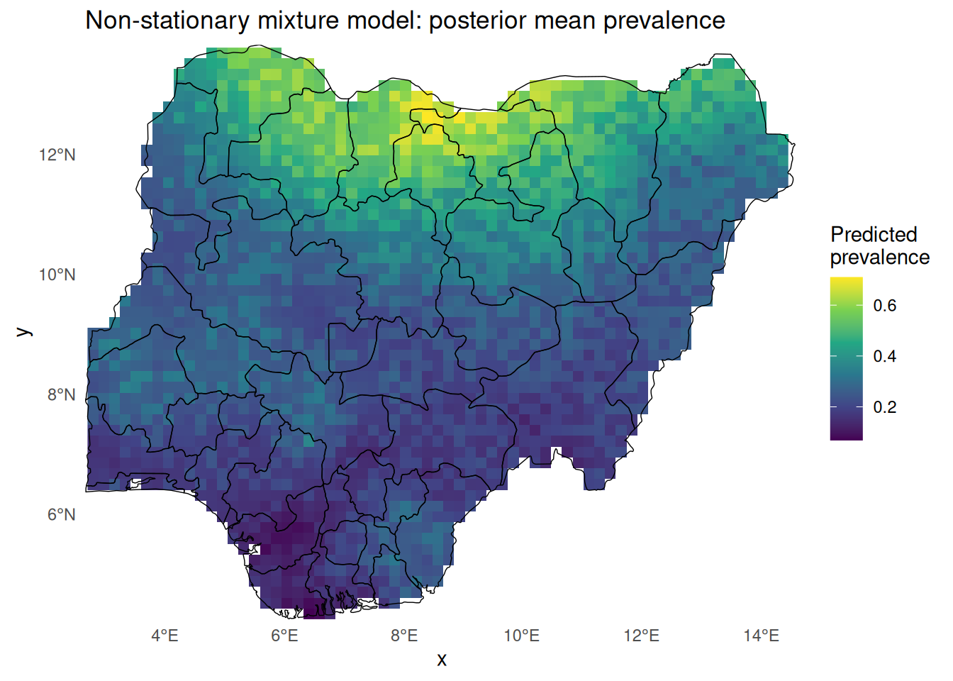
18. Predict and map (clipped to Nigeria)

Code

pred_grid_ns <- read_csv("data/prediction_grid_utm.csv") %>% 
mutate(w = (utm_y - min(utm_y)) / (max(utm_y) - min(utm_y)),
w = pmin(pmax(w, 0), 1)) %>%
st_as_sf(coords=c("utm_x","utm_y"), crs=32632)


pred_ns_sf <- predict(fit_ns, newdata = pred_grid_ns, n.samples = 200,
                      formula = ~ plogis(Intercept + elevation + ndvi + urban +
w*smooth + (1-w)*rough)) |>
rename(prev_mean = mean)
pred_ns_rast <- st_rasterize(pred_ns_sf["prev_mean"], dx = 20000, dy = 20000)
pred_ns_rast_ng <- pred_ns_rast[st_union(nga_admin1)]

ggplot() +
geom_stars(data = pred_ns_rast_ng, na.rm = TRUE) +
geom_sf(data = nga_admin1, fill = NA, colour = "black", linewidth = 0.25) +
coord_sf(expand = FALSE) +
scale_fill_viridis_c(name = "Predicted\nprevalence", na.value = NA) +
theme_minimal() +
theme(panel.grid = element_blank(),
panel.background = element_rect(fill = "white", colour = NA),
plot.background  = element_rect(fill = "white", colour = NA)) +
labs(title = "Non-stationary mixture model: posterior mean prevalence")

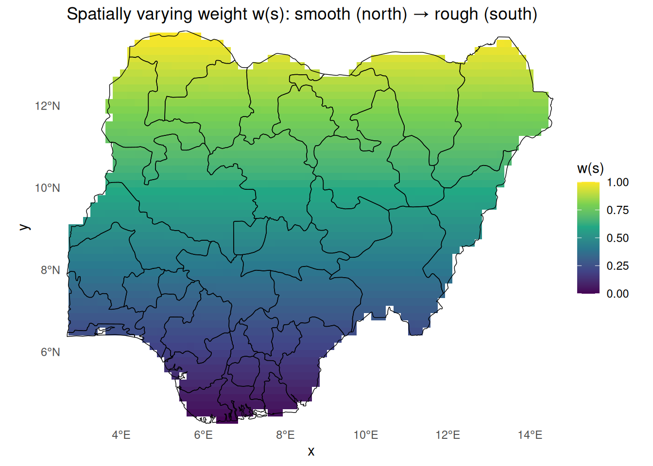
19. (Optional) Visualise the weight surface \(\omega(s)\)

Code

w_rast <- st_rasterize(pred_ns_sf["w"], dx = 20000, dy = 20000)[st_union(nga_admin1)]

ggplot() +
geom_stars(data = w_rast, na.rm = TRUE) +
geom_sf(data = nga_admin1, fill = NA, colour = "black", linewidth = 0.25) +
coord_sf(expand = FALSE) +
scale_fill_viridis_c(name = "w(s)", limits = c(0, 1), na.value = NA) +
theme_minimal() +
theme(panel.grid = element_blank(),
panel.background = element_rect(fill = "white", colour = NA),
plot.background  = element_rect(fill = "white", colour = NA)) +
labs(title = "Spatially varying weight w(s): smooth (north) → rough (south)")

============================================================

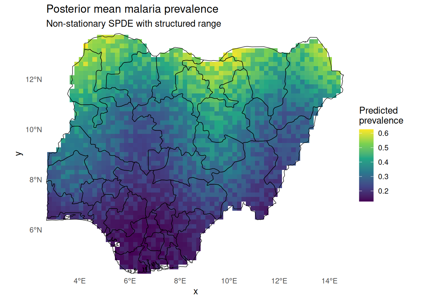
Part 1B — Non-stationary SPDE with structured range

============================================================

Here we make the SPDE range depend on a covariate at the mesh vertices by modelling log(kappa(s)) as: \[\log(\kappa(s)) = \theta_0 + \theta_1 z(s)\] and since range(s) = \(\sqrt(8)/\kappa(s)\), this gives a spatially varying range.

20. Mesh + vertex covariate

Use something interpretable like northing (y) or a “ecological gradient”.

Code

# Mesh for nonstationary dataset
coords_ns <- st_coordinates(nonstat_malaria_sf)

mesh_ns <- inla.mesh.2d(
  loc = coords_ns,
  max.edge = c(80000, 250000),
  cutoff   = 20000,
  offset   = c(100000, 200000)
)

# Vertex covariate: scaled northing at mesh vertices
z_vert <- scale(mesh_ns$loc[,2])[,1]   # mesh vertex y coordinate (UTM northing)

# Basis matrices for spatially varying kappa and/or tau
# Here: 2 hyperparameters for kappa: intercept + slope*z
B_kappa <- cbind(1, z_vert)

# Keep tau constant (1 parameter) OR also vary it; here constant:
B_tau <- matrix(1, nrow = nrow(B_kappa), ncol = 1)

21. Build B.tau / B.kappa with 4 columns

Here we use the Lindgren/Rue parameterisation.

Code

nu <- 1
alpha <- nu + 2/2

# constants for the SPDE parameterisation (same approach as the book)
logkappa0 <- log(8 * nu) / 2

logtau0 <- (lgamma(nu) - lgamma(alpha) - log(4*pi)) / 2
logtau0 <- logtau0 - logkappa0

B_tau   <- cbind(logtau0,  -1,  nu,  nu * z_vert)
B_kappa <- cbind(logkappa0, 0,  -1, -1 * z_vert)

22. Build a non-stationary SPDE using inla.spde2.matern

We specify priors for the theta parameters. (These are on log-scales internally.)

Code

spde_ns <- inla.spde2.matern(
  mesh = mesh_ns,
  B.kappa = B_kappa,
  B.tau   = B_tau,
  theta.prior.mean = c(log(1/300000), 0, 0),   # (kappa intercept), (kappa slope), (tau intercept)
  theta.prior.prec = c(1, 1, 1)                # weak-ish priors, Increasing theta.prior.prec tightens the prior (less variation).
  # The seco4)  Predict and mapnd entry in theta.prior.mean / prec controls how strongly the range can vary with z.
)

23. Fit binomial model with this structured-range SPDE

Code

cmp_ns_struct <- y ~
  1 + elevation + ndvi + urban +
  field_ns(geometry, model = spde_ns)

fit_ns_struct <- bru(
  components = cmp_ns_struct,
  family = "binomial",
  data = ns_dat,
  Ntrials = ns_dat$n_tested,
  options = list(control.compute = list(dic = TRUE, waic = TRUE))
)

summary(fit_ns_struct)

inlabru version: 2.13.0.9024 
INLA version: 25.12.02 
Latent components:
elevation: main = linear(elevation)
ndvi: main = linear(ndvi)
urban: main = linear(urban)
field_ns: main = spde(geometry)
Intercept: main = linear(1)
Observation models:
  Model tag: <No tag>
    Family: 'binomial'
    Data class: 'sf', 'tbl_df', 'tbl', 'data.frame'
    Response class: 'numeric'
    Predictor: y ~ elevation + ndvi + urban + field_ns + Intercept
    Additive/Linear/Rowwise: TRUE/TRUE/TRUE
    Used components: effect[elevation, ndvi, urban, field_ns, Intercept], latent[] 
Time used:
    Pre = 0.768, Running = 1.69, Post = 0.553, Total = 3.01 
Fixed effects:
            mean    sd 0.025quant 0.5quant 0.975quant   mode kld
elevation -0.001 0.000     -0.002   -0.001     -0.001 -0.001   0
ndvi       2.963 0.067      2.831    2.963      3.094  2.963   0
urban      0.265 0.024      0.219    0.265      0.311  0.265   0
Intercept -1.700 0.086     -1.867   -1.700     -1.532 -1.700   0

Random effects:
  Name    Model
    field_ns SPDE2 model

Model hyperparameters:
                      mean   sd 0.025quant 0.5quant 0.975quant   mode
Theta1 for field_ns -12.61 1.00     -14.58   -12.61     -10.64 -12.61
Theta2 for field_ns   0.00 1.00      -1.97     0.00       1.97   0.00
Theta3 for field_ns   0.00 1.00      -1.97     0.00       1.97   0.00

Deviance Information Criterion (DIC) ...............: 3488.63
Deviance Information Criterion (DIC, saturated) ....: 2011.74
Effective number of parameters .....................: 4.00

Watanabe-Akaike information criterion (WAIC) ...: 3514.04
Effective number of parameters .................: 28.89

Marginal log-Likelihood:  -1773.36 
 is computed 
Posterior summaries for the linear predictor and the fitted values are computed
(Posterior marginals needs also 'control.compute=list(return.marginals.predictor=TRUE)')

24. Predict and map

Code

pred_ns_sf <- predict(fit_ns_struct, newdata = pred_grid_ns, n.samples = 200, 
                      ~ plogis(Intercept + elevation + ndvi + urban + field_ns)) |>
  rename(prev_mean = mean)

pred_rast <- st_rasterize(pred_ns_sf["prev_mean"], dx = 20000, dy = 20000)
pred_rast_ng <- pred_rast[st_union(nga_admin1)]   # mask outside Nigeria

# --- (D) Plot ---
ggplot() +
  geom_stars(data = pred_rast_ng, na.rm = TRUE) +
  geom_sf(data = nga_admin1, fill = NA, colour = "black", linewidth = 0.25) +
  coord_sf(expand = FALSE) +
  scale_fill_viridis_c(name = "Predicted\nprevalence", na.value = NA) +
  theme_minimal() +
  theme(
    panel.grid = element_blank(),
    panel.background = element_rect(fill = "white", colour = NA),
    plot.background  = element_rect(fill = "white", colour = NA)
  ) +
  labs(
    title = "Posterior mean malaria prevalence",
    subtitle = "Non-stationary SPDE with structured range"
  )

Summary (Day 2)

Joint model: shared + group-specific spatial structure, two outcomes in one model

Non-stationary model: mixture of SPDEs with a spatially varying weight and structured range.

Mapping: predictions rasterised and clipped to Nigeria boundary