1. Spatial disease mapping with SDALGCP2

This tutorial fits a spatial disease-mapping model end to end. Every code block runs as shown, using the bundled example dataset sdalgcp_data so you can copy-paste and reproduce it exactly.

The model

We observe disease counts $Y_i$ aggregated over areal units $A_i$ ( $i=1,\dots,N$ ) with an offset $m_i$ (the expected count, e.g. population times a baseline rate). SDALGCP2 fits a spatially discrete approximation to a log-Gaussian Cox process: $Y_i \mid S \;\sim\; \mathrm{Poisson}\!\big(m_i\, e^{\eta_i}\big), \qquad \eta_i \;=\; d_i^\top\beta \;+\; S_i,$ where $d_i$ are area-level covariates and $S=(S_1,\dots,S_N)$ is a Gaussian spatial random effect. $S_i$ is the average over area $A_i$ of a continuous Gaussian process $S(x)$ with exponential covariance $\mathrm{Cov}\{S(x),S(x')\}=\sigma^2\exp(-\lVert x-x'\rVert/\phi)$ ; aggregating this process over the areas gives an $N\times N$ covariance built from candidate points inside each region (see Tutorial 4). The parameters are the coefficients $\beta$ , the spatial variance $\sigma^2$ and the range $\phi$ .

Two quantities are reported for every area:

Relative risk $\mathrm{RR}_i=e^{\eta_i}=e^{d_i^\top\beta+S_i}$ — the full relative risk, including the covariate effect (the relative_risk column);
Covariate-adjusted relative risk $\mathrm{RR}^{\mathrm{adj}}_i=e^{S_i}$ — the residual spatial relative risk after adjusting for covariates (where is risk high/low beyond what the covariates explain?) — the adjusted_rr column.

The data

sdalgcp() takes an sf object whose columns hold the response, covariates and offset. The package ships a small simulated example, sdalgcp_data: 64 regions with a disease count (cases), a covariate (x1), and a population offset (pop). It was generated with a true covariate effect of 0.6 and a baseline log-rate of -6, so we can check the model recovers them.

library(SDALGCP2)
library(sf)
#> Linking to GEOS 3.12.1, GDAL 3.8.4, PROJ 9.4.0; sf_use_s2() is TRUE

data(sdalgcp_data)
head(sdalgcp_data)
#> Simple feature collection with 6 features and 4 fields
#> Geometry type: POLYGON
#> Dimension:     XY
#> Bounding box:  xmin: 0 ymin: 0 xmax: 15 ymax: 2.5
#> CRS:           NA
#>   region cases          x1  pop                       geometry
#> 1      1     2 -2.03331626 3840 POLYGON ((0 0, 2.5 0, 2.5 2...
#> 2      2     3 -1.64601792 3985 POLYGON ((2.5 0, 5 0, 5 2.5...
#> 3      3     1 -1.25871959 2236 POLYGON ((5 0, 7.5 0, 7.5 2...
#> 4      4     0 -0.87142125  846 POLYGON ((7.5 0, 10 0, 10 2...
#> 5      5     3 -0.48412292  874 POLYGON ((10 0, 12.5 0, 12....
#> 6      6    12 -0.09682458 2231 POLYGON ((12.5 0, 15 0, 15 ...

# crude standardised incidence ratio (SIR): observed / expected-at-overall-rate
rate <- sum(sdalgcp_data$cases) / sum(sdalgcp_data$pop)
sdalgcp_data$SIR <- sdalgcp_data$cases / (sdalgcp_data$pop * rate)

The crude SIR is noisy and over-fits sparsely populated areas — exactly what a model smooths:

plot(sdalgcp_data["SIR"], main = "Crude SIR (the data)")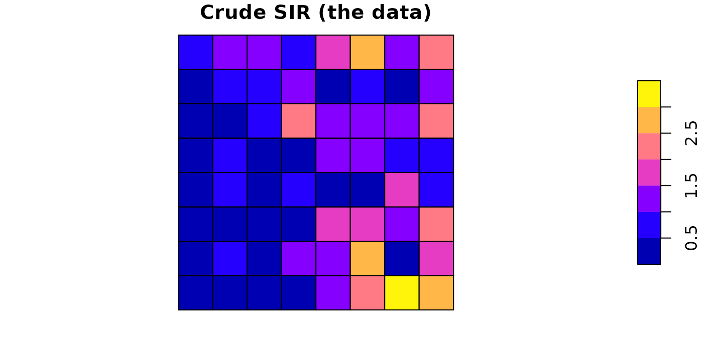

plot(sdalgcp_data["x1"],  main = "Covariate x1")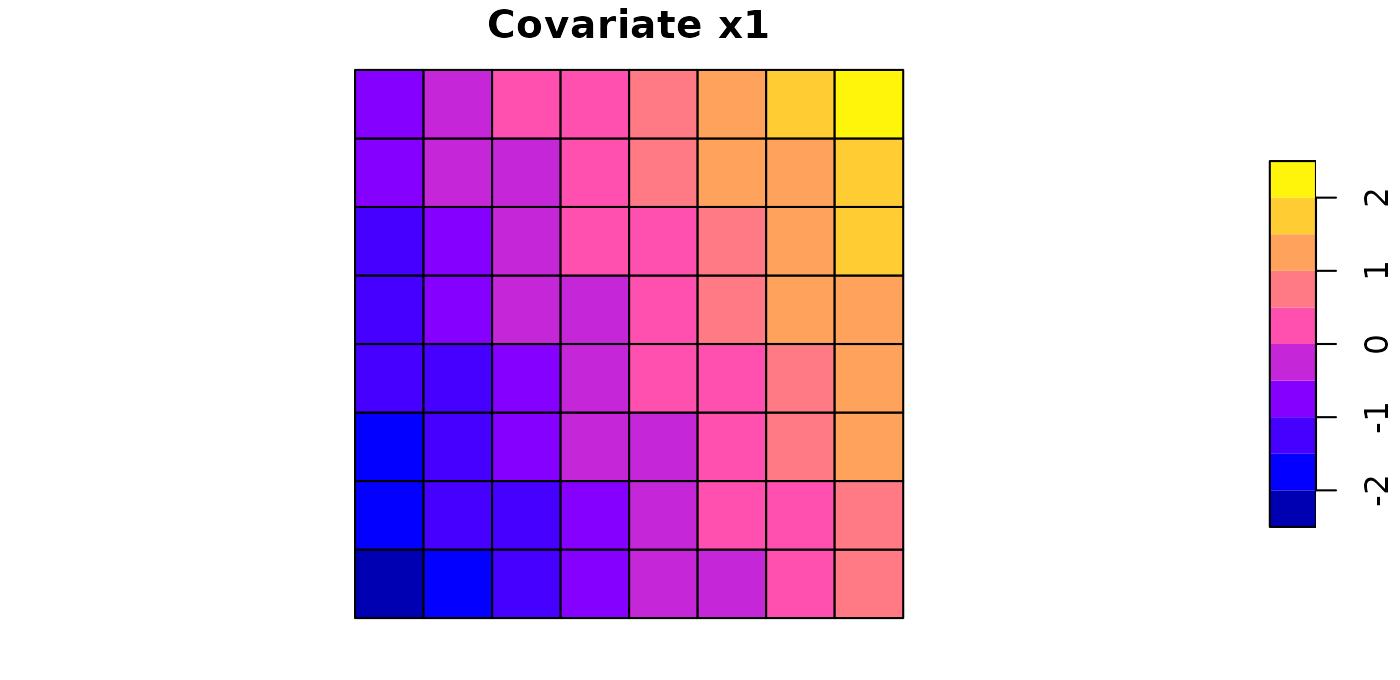

Fit

One call. Candidate-point spacing, the spatial range and MCMC settings are chosen automatically; reanchor re-simulates the latent field at the optimum a couple of times for reliable variance estimates. (We set a seed and a shorter MCMC run here so the vignette is quick and reproducible; the defaults are longer.)

set.seed(2024)
fit <- sdalgcp(cases ~ x1 + offset(log(pop)), data = sdalgcp_data,
               control = sdalgcp_control(n_sim = 4000, burnin = 1000, thin = 5,
                                         reanchor = 1))
summary(fit)
#> Call: sdalgcp(formula = cases ~ x1 + offset(log(pop)), data = sdalgcp_data, 
#>     control = sdalgcp_control(n_sim = 4000, burnin = 1000, thin = 5, 
#>         reanchor = 1))
#> 
#> Coefficients:
#>             Estimate Std.Err z value Pr(>|z|)    
#> (Intercept)   -6.226   0.143  -43.55  < 2e-16 ***
#> x1             0.660   0.136    4.84  1.3e-06 ***
#> sigma^2        0.876   0.378    2.32    0.021 *  
#> phi            1.207   0.448    2.69    0.007 ** 
#> ---
#> Signif. codes:  0 '***' 0.001 '**' 0.01 '*' 0.05 '.' 0.1 ' ' 1
#> 
#> Spatial scale phi: 1.20698
#> Log-likelihood: 0.574661
#> MC importance-sampling ESS: 102 / 600 (17%);  log-lik MC SE: 0.0902
#> Note: sigma^2 is the variance of the latent Gaussian process.

The covariate effect x1 is estimated close to its true value of 0.6, the spatial range phi and variance sigma^2 describe the residual spatial structure, and the importance-sampling effective sample size reports how reliable the Monte Carlo likelihood is.

Map the two relative risks

plot(fit, "relative_risk")   # relative risk exp(d'beta + S)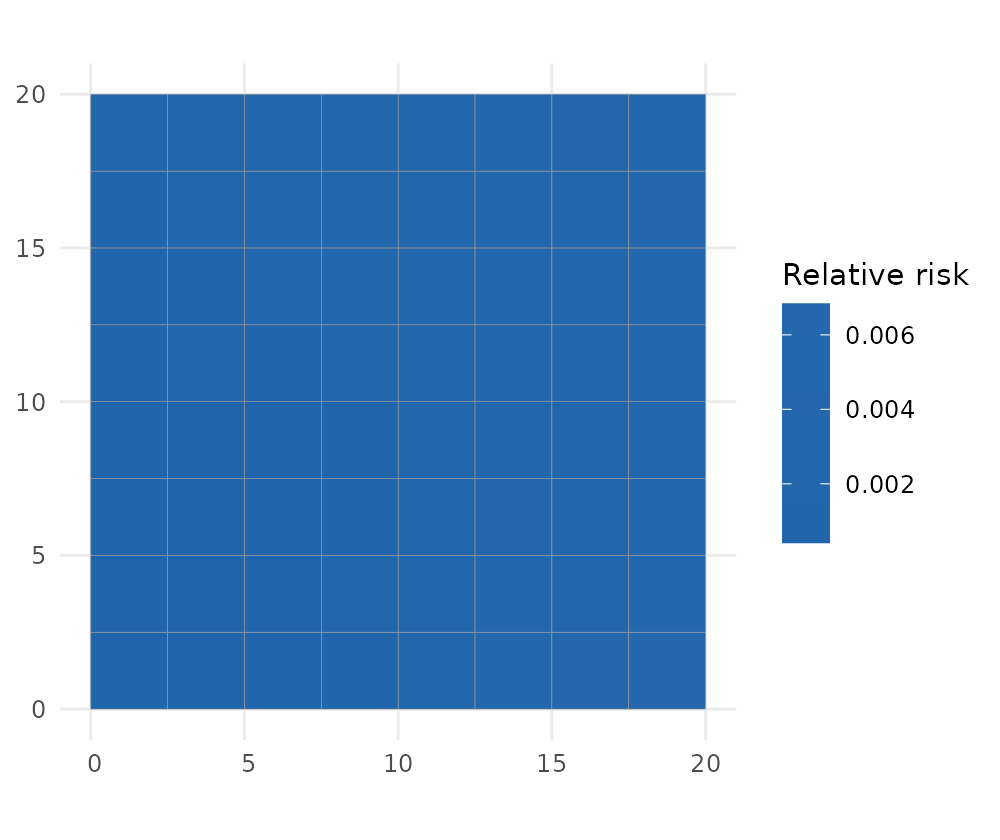

plot(fit, "adjusted_rr")     # covariate-adjusted relative risk exp(S)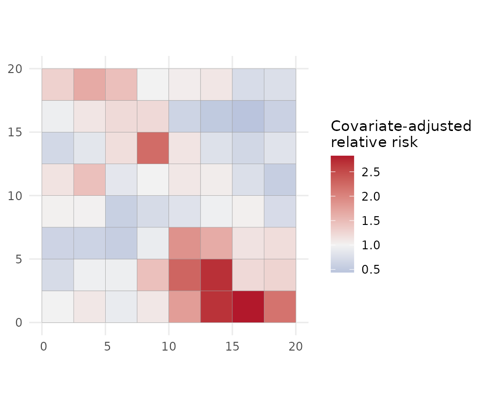

relative_risk (left) is the overall pattern of risk; adjusted_rr (right) strips out the covariate contribution and shows the unexplained spatial signal — useful for spotting hotspots that the covariates do not account for.

Uncertainty and exceedance

Every quantity comes with a standard error, and you can ask for the probability that risk exceeds a policy threshold:

plot(fit, "adjusted_rr_se")                  # standard error of the adjusted RR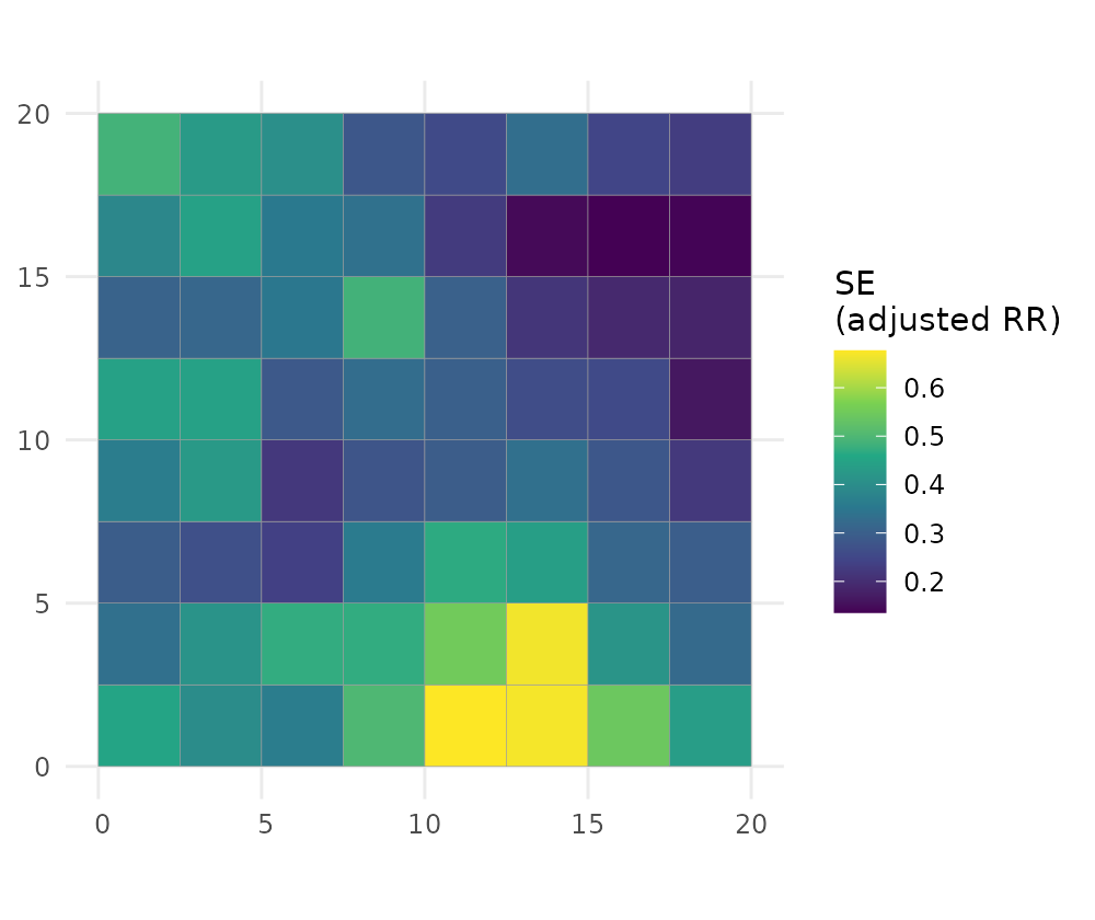

plot(fit, "exceedance", threshold = 1.5)     # P(adjusted RR > 1.5)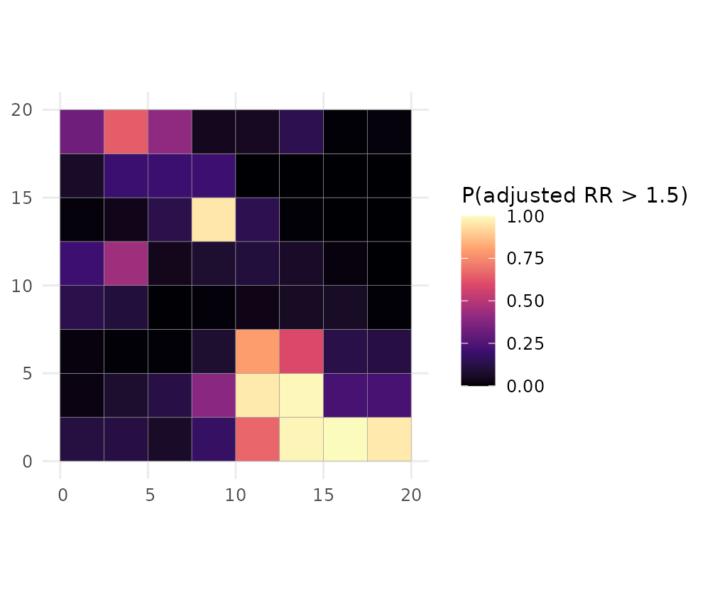

The exceedance map is usually the most decision-relevant output: it flags areas that are confidently above the threshold rather than high by chance. By default the exceedance is computed for the covariate-adjusted relative risk (which = "adjusted_rr"); pass which = "relative_risk" for the full relative risk instead.

A continuous surface

Risk can also be predicted on a fine grid (change-of-support), giving a smooth surface instead of a choropleth:

pc <- predict(fit, type = "continuous", sampler = "laplace", cellsize = 1)
plot(pc, "adjusted_rr", bound = sdalgcp_data)
#> Coordinate system already present.
#> ℹ Adding new coordinate system, which will replace the existing one.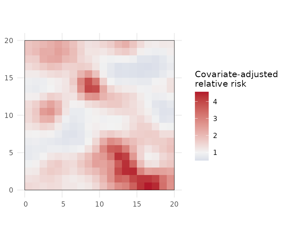

predict() returns an sf with all four quantities (relative_risk, adjusted_rr and their _se) for both type = "discrete" and type = "continuous", and exceedance() works on either.

Model checking

Finally, check that the spatial term has absorbed the spatial structure: the Pearson residuals should show no leftover spatial autocorrelation.

chk <- model_check(fit)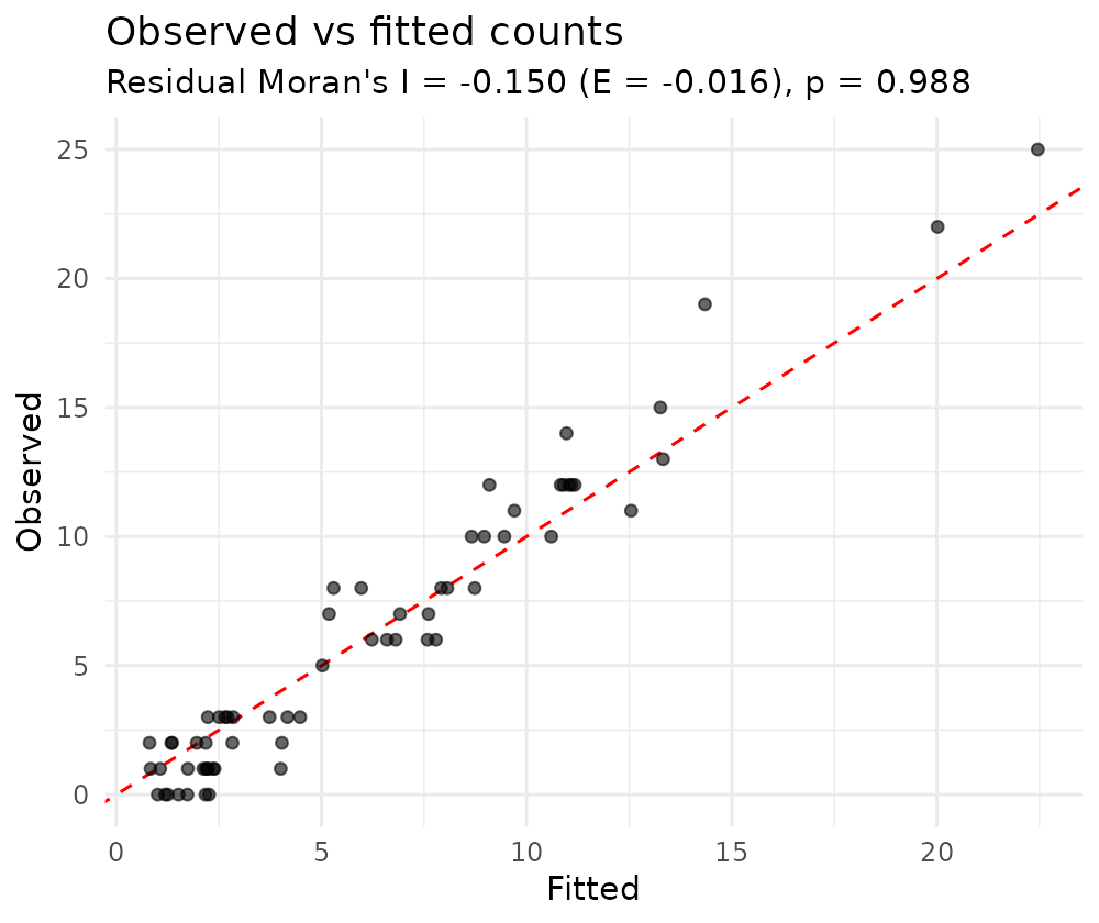

chk$moran   # residual Moran's I and its permutation p-value
#> $I
#> [1] -0.1501438
#> 
#> $expected
#> [1] -0.01587302
#> 
#> $p_value
#> [1] 0.988

A non-significant residual Moran’s I indicates the model has captured the spatial pattern, and the observed-vs-fitted points lie around the identity line.

Real data

sdalgcp_data is simulated so we know the truth. For a real example, the package also ships liver — incident primary biliary cirrhosis counts by LSOA in North East England (Johnson et al. 2019), which you can fit the same way:

data(liver)
fit_liver <- sdalgcp(cases ~ IMD + offset(log(pop)), data = liver)
plot(fit_liver, "relative_risk")

Raster predictors — continuous covariates done right.
Spatio-temporal — space–time relative risk.
Estimating the scale — what $\phi$ is and how it is estimated.
Spatial confounding and misaligned covariates.