5. Spatial confounding and restricted spatial regression • SDALGCP2

When a covariate is itself spatially structured (a north–south gradient, deprivation, distance to a city), it is collinear with the spatial random effect: the data can be explained almost equally well by “covariate effect” or by “spatial noise”. This is spatial confounding. This tutorial is self-contained and deliberately balanced — spatial confounding is a genuinely nuanced topic.

The issue

The model is $\eta_i=d_i^\top\beta+S_i$ with $S\sim\mathcal N(0,\sigma^2 R(\phi))$ . When a column of $d$ lies close to the leading spatial modes of $R(\phi)$ , the coefficient $\beta$ and the random effect $S$ compete to explain the same pattern. The consequence is that $\widehat\beta$ is poorly identified — uncertain, and sensitive to how the spatial term is specified.

Restricted spatial regression (RSR)

One remedy (Reich, Hodges & Zadnik 2006; Hughes & Haran 2013) constrains the random effect to the orthogonal complement of the fixed-effect design. With $K$ an orthonormal basis of $\mathrm{null}(D^\top)$ , the model becomes $\eta=D\beta+K\alpha,\qquad \alpha\sim\mathcal N\!\big(0,\sigma^2 K^\top R(\phi)K\big),$ so $K\alpha$ cannot reproduce any column of $D$ and $\beta$ is identified by the data, not by the spatial smoothing. SDALGCP2 fits it by a Laplace-approximate marginal likelihood (derivation: math/confounding-and-misalignment.pdf).

library(SDALGCP2)
library(sf)

set.seed(2)
regions <- st_sf(geometry = st_make_grid(
  st_as_sfc(st_bbox(c(xmin = 0, ymin = 0, xmax = 20, ymax = 20))), n = c(8, 8)))
N <- nrow(regions)
pts <- sda_points(regions, delta = 1.2, method = 3)
S   <- as.numeric(t(chol(0.7 * precompute_corr(pts, 4)$R[, , 1])) %*% rnorm(N))
regions$x1    <- as.numeric(scale(st_coordinates(st_centroid(regions))[, 1]))  # spatial gradient
regions$pop   <- round(runif(N, 500, 3000))
regions$cases <- rpois(N, regions$pop * exp(-6 + 0.6 * regions$x1 + S))

# standard fit vs restricted spatial regression
fit_std <- sdalgcp(cases ~ x1 + offset(log(pop)), regions)
fit_rsr <- sdalgcp(cases ~ x1 + offset(log(pop)), regions,
                   control = sdalgcp_control(confounding = "restricted"))

What RSR does — and what it does not

Because the single-dataset estimate depends on the (random) alignment of the spatial field with the covariate, the honest way to see the effect is a small simulation study — 24 data sets generated as above (true $\beta=0.6$ ), fitting both methods:

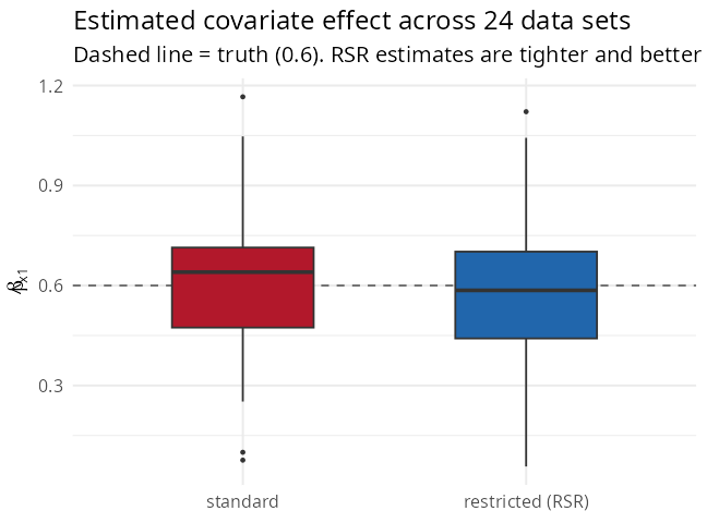
#> Across 24 simulated data sets (true beta = 0.6):
#>   standard          mean est = 0.602,  SD of est = 0.265,  mean SE = 0.151
#>   restricted (RSR)  mean est = 0.587,  SD of est = 0.267,  mean SE = 0.074

Two things stand out:

both methods are essentially unbiased on average (0.60 vs 0.59) — here the spatial term is genuine noise, not a hidden confounder, so neither systematically attenuates $\beta$ ;
RSR reports a much smaller standard error (0.074 vs 0.151). Its estimate is identified purely by the within-covariate signal, so it looks very precise.

Caveat (important). That small RSR standard error can be anti-conservative: it does not reflect the across-data-set spread ( $\approx0.27$ here), because it treats the spatial–covariate separation as known. This is the well-documented critique of RSR (Hanks et al. 2015; Zimmerman & Ver Hoef 2021). Whether RSR helps depends on the causal role of the spatial term: if it is just smooth noise, RSR gives a clean, data-driven estimate; if it is a proxy for an unmeasured spatial confounder, the unrestricted model may actually be preferable.

Practical guidance

Use confounding = "restricted" when you want a coefficient identified by the covariate’s own variation, free of the spatial smoothing — but treat its standard error as a lower bound.
When covariates are non-spatial (e.g. an individual-level rate), confounding is not a concern and the default fit is appropriate.
In all cases, report which choice you made: the spatial term and the covariate are partly interchangeable, and that is a property of the data, not a bug.

References

Reich, Hodges & Zadnik (2006) Biometrics; Hughes & Haran (2013) JRSS-B; Hanks, Schliep, Hooten & Hoeting (2015) Environmetrics; Zimmerman & Ver Hoef (2021) Spatial Statistics. ```