4. Estimating the spatial scale: grid vs continuous

The spatial scale $\phi$ controls how fast spatial correlation decays with distance — it sets the “reach” of a hotspot. This tutorial explains how SDALGCP2 estimates it and is self-contained.

Where $\phi$ lives: a double integral

The region-level random effect $S_i$ is the average over area $A_i$ of a continuous process $S(x)$ with $\mathrm{Cov}\{S(x),S(x')\}=\sigma^2 e^{-\lVert x-x'\rVert/\phi}$ . The covariance between two regions is therefore a double integral over the pair of areas: $R_{ij}(\phi)=\int_{A_i}\!\int_{A_j} w_i(x)\,w_j(y)\, \exp\!\Big(-\tfrac{\lVert x-y\rVert}{\phi}\Big)\,dx\,dy,$ approximated by a weighted sum over the candidate points inside each region. $\phi$ appears inside this integral, so the whole $N\times N$ correlation matrix depends on it. There are two ways to estimate it.

Set up an example

library(SDALGCP2)
library(sf)

set.seed(11)
regions <- st_sf(geometry = st_make_grid(
  st_as_sfc(st_bbox(c(xmin = 0, ymin = 0, xmax = 20, ymax = 20))), n = c(9, 9)))
N <- nrow(regions)
pts <- sda_points(regions, delta = 1.1, method = 3)
S   <- as.numeric(t(chol(0.5 * precompute_corr(pts, 3)$R[, , 1])) %*% rnorm(N))  # true phi = 3
regions$x1    <- rnorm(N)
regions$pop   <- round(runif(N, 800, 4000))
regions$cases <- rpois(N, regions$pop * exp(-6 + 0.5 * regions$x1 + S))

Grid (profile)

The classic approach: evaluate the model on a grid of $\phi$ values and take the profile maximum.

fit_grid <- sdalgcp(cases ~ x1 + offset(log(pop)), data = regions,
                    control = sdalgcp_control(scale = "grid",
                                              phi = seq(1.5, 6, length.out = 12)))

Continuous (direct) — the default

The aggregated correlation $R(\phi)$ is differentiable in $\phi$ : the derivative is obtained by differentiating the kernel inside the integral, $\partial_\phi e^{-d/\phi}=e^{-d/\phi}\,d/\phi^2$ . SDALGCP2 therefore optimises $\phi$ directly, jointly with $\beta$ and $\sigma^2$ , with no grid. This removes the grid-discretisation error and — because $\phi$ is now a fitted parameter — yields a proper standard error from the joint Hessian (full derivation: math/continuous-phi-derivation.pdf).

fit_dir <- sdalgcp(cases ~ x1 + offset(log(pop)), data = regions)  # scale = "continuous"

They agree — and continuous gives a standard error

# (timings will vary)

#> GRID:       phi = 2.73            beta_x1 = 0.437   [6.0s]
#> CONTINUOUS: phi = 2.86 (SE 0.35)  beta_x1 = 0.449   [6.2s]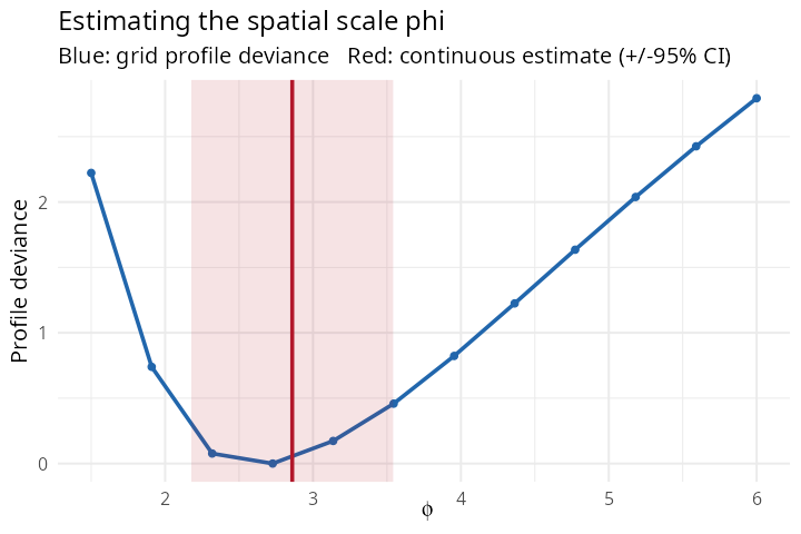

The blue curve is the grid profile deviance; its minimum (the grid $\hat\phi$ ) falls between grid nodes. The red line is the continuous estimate with its 95% confidence band — essentially the same value, but obtained without choosing a grid and with an honest standard error that the grid cannot provide.

Which to use?

	grid	continuous (default)
$\hat\phi$	restricted to grid nodes	exact, no discretisation error
SE for $\phi$	not available	from the joint Hessian
profile shape	fully visible (good for multimodality)	not traced
Matérn smoothness	any	0.5, 1.5, 2.5

Use continuous (the default) for a clean estimate with a standard error and no grid to choose. Use grid when you want to inspect the whole profile — e.g. to check for a flat or multimodal likelihood, with plot(fit_grid). Both are selected by sdalgcp_control(scale = ...). ```

Where ϕ\phi lives: a double integral