2. Spatially continuous (raster) predictors • SDALGCP2

A covariate often varies within each areal unit — elevation, distance to a road, pollution from point sources. The usual shortcut is to average it over each polygon and put the average into a Poisson model. Under the nonlinear log link this is biased. This tutorial shows why, and how SDALGCP2 does it correctly. It is self-contained.

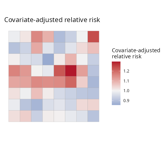
The problem, precisely

A region’s expected count under the log-Gaussian Cox process is $\mathbb{E}[Y_i\mid S] \;=\; m_i\int_{A_i} w_i(x)\,\exp\{z(x)^\top\beta + S(x)\}\,dx \;\approx\; m_i\sum_{k} w_{ik}\,\exp\{z(x_{ik})^\top\beta + S(x_{ik})\},$ a sum over candidate points $x_{ik}$ inside $A_i$ with weights $w_{ik}$ . The covariate enters inside the exponential. Factor it out: $\mathbb{E}[Y_i\mid S] \;\approx\; m_i\,e^{\,b_i(\beta)}\sum_k c_{ik}\,e^{S(x_{ik})}, \qquad \boxed{\,b_i(\beta)=\log\sum_k w_{ik}\,\exp\{z(x_{ik})^\top\beta\}\,}$ The region’s covariate contribution is the log-sum-exp $b_i(\beta)$ , not $(\bar z_i)^\top\beta$ with $\bar z_i$ the areal mean. By Jensen’s inequality the two differ whenever $z$ varies within the region, and a regression on $\bar z_i$ is biased for $\beta$ — badly so when sharp features (e.g. point sources) sit inside regions. Full derivation: math/raster-covariates-derivation.pdf.

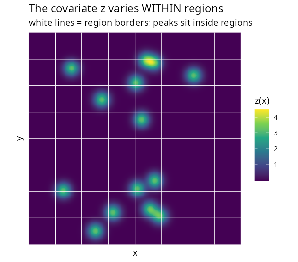
The data

A covariate z with sharp peaks (think pollution sources), supplied as a terra::SpatRaster, plus outcome counts over an 8×8 lattice. The peaks sit inside regions, so the region mean loses them:

library(SDALGCP2)
library(sf)
library(terra)

set.seed(3)
# a raster covariate with 14 sharp Gaussian peaks
r <- rast(xmin = 0, xmax = 20, ymin = 0, ymax = 20, resolution = 0.08)
xy  <- xyFromCell(r, 1:ncell(r))
src <- matrix(runif(2 * 14, 1, 19), ncol = 2)
values(r) <- rowSums(sapply(seq_len(nrow(src)), function(s)
  3.2 * exp(-((xy[, 1] - src[s, 1])^2 + (xy[, 2] - src[s, 2])^2) / 0.5)))
names(r) <- "z"

sh <- st_sf(geometry = st_make_grid(
  st_as_sfc(st_bbox(c(xmin = 0, ymin = 0, xmax = 20, ymax = 20))), n = c(8, 8)))
N <- nrow(sh)

# simulate counts from the point-level intensity model (true beta_z = 1)
pts <- sda_points(sh, delta = 0.5, method = 3); w <- lapply(pts, function(p) p$weight)
Z   <- lapply(pts, function(p) cbind(1, terra::extract(r, as.matrix(p$xy))[, "z"]))
b_true <- sapply(seq_len(N), function(i) log(sum(w[[i]] * exp(as.numeric(Z[[i]] %*% c(-6, 1))))))
sh$pop   <- round(runif(N, 2000, 6000))
sh$cases <- rpois(N, sh$pop * exp(b_true))
sh$zbar  <- sapply(seq_len(N), function(i) sum(w[[i]] * Z[[i]][, 2]))  # areal mean

The raster covariate (varies within regions)	What areal averaging keeps

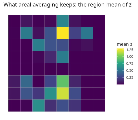The right panel — the region mean — has washed the peaks out.

Fitting: naive vs intensity-scale

The naive analysis regresses counts on the areal mean:

naive <- glm(cases ~ zbar + offset(log(pop)), poisson, st_drop_geometry(sh))
coef(naive)["zbar"]
#> 1.67   <- 67% too large

SDALGCP2 instead reads z from the raster at the candidate points and uses the log-sum-exp offset. Pass the raster; sh does not even need a z column:

fit <- sdalgcp(cases ~ z + offset(log(pop)), data = sh, rasters = r)
coef(naive)["zbar"]; fit$beta_opt["z"]

#> Estimate of beta_z:
#>   truth                       1.00
#>   naive areal average         1.67   (+67% bias)
#>   SDALGCP2 (intensity-scale)  1.09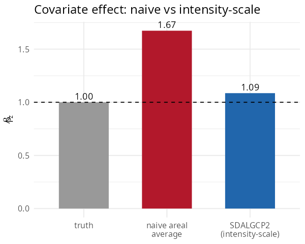

Averaging the predictor over polygons overstates the effect by two-thirds; aggregating on the intensity scale recovers it.

When does it matter?

Because $b_i(\beta)\approx\bar z_i^\top\beta+\tfrac12\beta^\top\widehat{\mathrm{Var}}_i(z)\beta$ , the bias is driven by the within-region variance of $z$ . It is large when that variance is correlated with the region mean — sharp, localised features such as point sources. For smooth covariates the two approaches nearly agree, and either is fine.

Output

As in Tutorial 1, the fit yields relative risk and covariate-adjusted relative risk with standard errors and exceedance, both discrete and continuous:

plot(fit, "adjusted_rr")                 # covariate-adjusted relative risk
plot(fit, "exceedance", threshold = 1.5)

Options

sdalgcp_control(tilt_spatial = TRUE) additionally tilts the spatial correlation by the covariate intensity (the fully tilted model of the PDF); the default keeps the correlation covariate-free and is faster. ```