3. Spatio-temporal disease mapping • SDALGCP2

When the same regions are observed at several times, add time = and SDALGCP2 fits a separable space–time model. This tutorial is self-contained.

The model

For region $i$ at time $t$ , counts $Y_{it}$ with offset $m_{it}$ : $Y_{it}\mid S \sim \mathrm{Poisson}\!\big(m_{it}\,e^{\eta_{it}}\big), \qquad \eta_{it}=d_{it}^\top\beta + S_{it},$ with a separable space–time covariance $\mathrm{Cov}(S_{it},S_{js}) \;=\; \sigma^2\,R_s(\lVert\cdot\rVert;\phi)_{ij}\;R_t(|t-s|;\nu)_{ts},$ i.e. $\mathrm{Cov}(\mathrm{vec}\,S)=\sigma^2\,(R_t(\nu)\otimes R_s(\phi))$ , where $R_s$ is the aggregated spatial correlation (range $\phi$ ) and $R_t$ a temporal Matérn correlation (range $\nu$ ). SDALGCP2 never forms the $(N\!\cdot\!T)\times(N\!\cdot\!T)$ covariance — it uses the Kronecker identities $x^\top(R_t\otimes R_s)^{-1}x=\mathrm{tr}(R_s^{-1}M R_t^{-1}M^\top)$ and $\log|R_t\otimes R_s|=N\log|R_t|+T\log|R_s|$ — so it scales to many regions and times. The temporal range $\nu$ is estimated alongside $\beta,\sigma^2,\phi$ .

The data

One row per region and time, with the geometry repeated. Here four years on a 6×6 lattice:

library(SDALGCP2)
library(sf)

set.seed(7)
shp <- st_sf(geometry = st_make_grid(
  st_as_sfc(st_bbox(c(xmin = 0, ymin = 0, xmax = 18, ymax = 18))), n = c(6, 6)))
N <- nrow(shp); times <- 2019:2022; T <- length(times)

# simulate separable space-time counts (true beta=0.5)
pts <- sda_points(shp, delta = 1.4, method = 3)
Rs  <- precompute_corr(pts, 3)$R[, , 1]
Rt  <- SDALGCP2:::.temporal_corr(seq_len(T), 1.5, 0.5)
L   <- t(chol(0.4 * kronecker(Rt, Rs)))
x1  <- rnorm(N * T); pop <- round(runif(N * T, 1000, 5000))
y   <- rpois(N * T, pop * exp(-6 + 0.5 * x1 + as.numeric(L %*% rnorm(N * T))))

dat <- st_sf(
  data.frame(cases = y, x1 = x1, pop = pop, year = rep(times, each = N)),
  geometry = st_geometry(shp)[rep(seq_len(N), T)])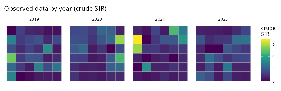

Fit

fit <- sdalgcp(cases ~ x1 + offset(log(pop)), data = dat, time = "year",
               control = sdalgcp_control(reanchor = 2))
summary(fit)

#> Coefficients:
#>             Estimate Std.Err z value Pr(>|z|)
#> (Intercept)  -6.167   0.107  -57.61   <2e-16 ***
#> x1            0.592   0.038   15.73   <2e-16 ***
#> sigma^2       0.491   0.205    2.39    0.017 *
#> nu            0.853   0.360    2.37    0.018 *
#>
#> Spatial scale phi: 2.02

nu is the temporal range (correlation length in years); phi the spatial range.

Predict and map — pick a year and a quantity

predict() returns a long sf — one row per region and time, with columns relative_risk, adjusted_rr and their standard errors (the same column names as the spatial predictor, so you can st_write() or map it directly). The plot() method selects a time and a quantity ("relative_risk", "adjusted_rr", "relative_risk_se", "adjusted_rr_se", "exceedance"):

pr <- predict(fit)

plot(pr, time = NULL, what = "adjusted_rr")          # facet all years
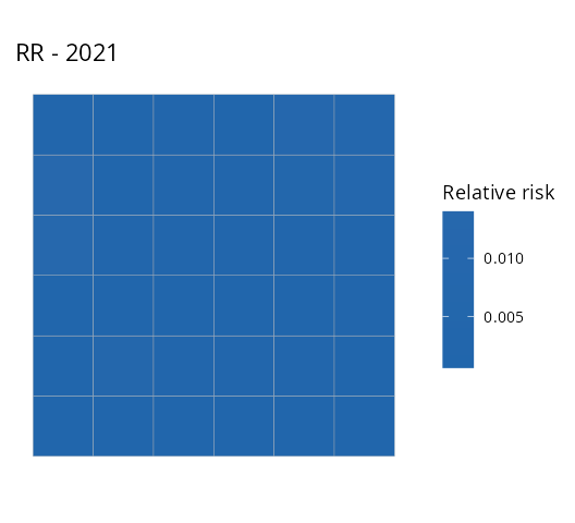
plot(pr, time = 2021, what = "relative_risk")        # relative risk, 2021 only
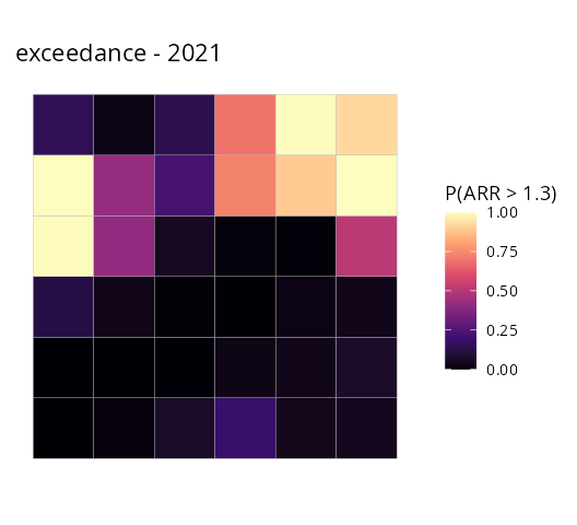
plot(pr, time = 2021, what = "exceedance", threshold = 1.3, which = "adjusted_rr")

Covariate-adjusted relative risk, all years:

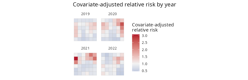
Relative risk, 2021	P(adjusted RR > 1.3), 2021

You can equally call plot(fit, time = 2021, what = "relative_risk") directly on the fit, and pr (the returned sf) is a long region × time table of every quantity for further analysis or mapping.

Covariates and confounding

The space–time model supports the same covariate extensions as the spatial one. The covariate surface is taken to be time-invariant (a covariate that genuinely changes over time can always go in as an ordinary data column); the intensity- scale tilting is then computed once per region and reused across the times, fitted by a Gauss–Newton loop around the space–time likelihood.

Raster (intensity-scale) covariates — a spatially continuous covariate supplied as a terra raster, aggregated correctly under the log link (see the raster tutorial):

library(terra)
fit_r <- sdalgcp(cases ~ elevation + offset(log(pop)), data = dat, time = "year",
                 rasters = elevation_raster)

Misaligned covariates — a covariate observed on a different (time-invariant) support, e.g. pollution monitors, kriged to the candidate points with a Berkson correction (see misaligned covariates):

fit_m <- sdalgcp(cases ~ pm25 + offset(log(pop)), data = dat, time = "year",
                 covariates = list(pm25 = monitors_sf))

Spatial confounding — when a covariate is spatially smooth it can be collinear with the random effect; restricted spatial regression de-confounds the coefficient (see spatial confounding). It generalises to space–time by constraining the random effect orthogonal to the design over all region–times:

fit_c <- sdalgcp(cases ~ x1 + offset(log(pop)), data = dat, time = "year",
                 control = sdalgcp_control(confounding = "restricted"))

The restricted space–time fit reduces exactly to the spatial restricted fit when there is a single time, and forms the full $(N\!\cdot\!T)\times(N\!\cdot\!T)$ covariance, so it is best suited to modest $N\!\cdot\!T$ .

Tips

Spatio-temporal fits profile the spatial range phi on a grid (set it with sdalgcp_control(phi = ...)); the temporal range nu is estimated continuously. Increase reanchor if the variance parameters look unstable. ```