Map an sdalgcp fit — plot.sdalgcp • SDALGCP2

Predicts and maps a chosen quantity. Works for spatial fits (discrete or continuous) and spatio-temporal fits (select a time).

Usage

# S3 method for class 'sdalgcp'
plot(
  x,
  what = c("relative_risk", "adjusted_rr", "relative_risk_se", "adjusted_rr_se",
    "exceedance"),
  type = c("discrete", "continuous"),
  time = NULL,
  threshold = 1,
  which = c("adjusted_rr", "relative_risk"),
  cellsize = NULL,
  sampler = c("mcmc", "laplace"),
  ...
)

Arguments

x: an "sdalgcp" fit.
what: one of "relative_risk" (relative risk, default), "adjusted_rr" (covariate-adjusted relative risk), "relative_risk_se", "adjusted_rr_se" or "exceedance".
type: "discrete" (default) or "continuous" (spatial fits).
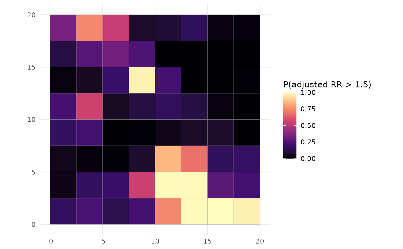
time: for spatio-temporal fits, the time to map (default: first; use NULL to facet all times).
threshold: threshold for what = "exceedance".
which: for exceedance: "adjusted_rr" (default) or "relative_risk".
cellsize: grid spacing for type = "continuous".
sampler: "mcmc" (default) or "laplace".
...: passed to the mapping layer.

Value

a ggplot object.

Examples

# \donttest{
data(sdalgcp_data)
fit <- sdalgcp(cases ~ x1 + offset(log(pop)), data = sdalgcp_data,
               control = sdalgcp_control(n_sim = 2000, burnin = 500, thin = 5,
                                         reanchor = 0))
plot(fit)                              # relative-risk map (predicts internally)

plot(fit, what = "exceedance", threshold = 1.5)

# }