Predict relative risk from a fitted SDALGCP2 model

Usage

# S3 method for class 'SDALGCP2'
predict(
  object,
  type = c("discrete", "continuous"),
  sampler = c("mcmc", "laplace"),
  cellsize = NULL,
  pred.loc = NULL,
  control.mcmc = NULL,
  ...
)

Arguments

object: an object of class "SDALGCP2" from SDALGCP2 or mcml_fit.
type: "discrete" for region-level inference or "continuous" for a spatially continuous surface.
sampler: "mcmc" (MALA, default) or "laplace" (fast Gaussian approximation, no MCMC).
cellsize: grid spacing for continuous prediction (ignored if pred.loc supplied).
pred.loc: optional data frame of prediction coordinates (x, y) for continuous prediction.
control.mcmc: optional MCMC controls; defaults to those used at fitting.
...: unused.

Value

an sf (class c("SDALGCP2_pred", "sf", "data.frame")) with one row per location – polygons for type = "discrete", grid-cell points for type = "continuous" – carrying the posterior mean and standard error of two relative-risk quantities:

relative_risk, relative_risk_se: the relative risk \(\exp(d'\beta + S)\) – the fitted risk relative to the offset baseline, combining the covariate effect and the residual spatial variation. This is the headline disease-mapping quantity.
adjusted_rr, adjusted_rr_se: the covariate-adjusted relative risk \(\exp(S)\) – the purely spatial relative risk that remains after holding the covariates fixed (the spatial signal the covariates do not explain).

The full posterior draws are retained as object attributes so that exceedance and map_exceedance can be computed for either quantity. Map a column with plot.SDALGCP2_pred.

Examples

# \donttest{
data(sdalgcp_data)
fit <- sdalgcp(cases ~ x1 + offset(log(pop)), data = sdalgcp_data,
               control = sdalgcp_control(n_sim = 2000, burnin = 500, thin = 5,
                                         reanchor = 0))

## region-level (discrete) prediction: an sf you can map or st_write()
pr <- predict(fit, type = "discrete")
head(pr)                       # relative_risk / adjusted_rr (+ standard errors)
#> Simple feature collection with 6 features and 8 fields
#> Geometry type: POLYGON
#> Dimension:     XY
#> Bounding box:  xmin: 0 ymin: 0 xmax: 15 ymax: 2.5
#> CRS:           NA
#>   region cases          x1  pop                       geometry relative_risk
#> 1      1     2 -2.03331626 3840 POLYGON ((0 0, 2.5 0, 2.5 2...  0.0005081073
#> 2      2     3 -1.64601792 3985 POLYGON ((2.5 0, 5 0, 5 2.5...  0.0007222510
#> 3      3     1 -1.25871959 2236 POLYGON ((5 0, 7.5 0, 7.5 2...  0.0007493540
#> 4      4     0 -0.87142125  846 POLYGON ((7.5 0, 10 0, 10 2...  0.0011510783
#> 5      5     3 -0.48412292  874 POLYGON ((10 0, 12.5 0, 12....  0.0024677851
#> 6      6    12 -0.09682458 2231 POLYGON ((12.5 0, 15 0, 15 ...  0.0050585377
#>   relative_risk_se adjusted_rr adjusted_rr_se
#> 1     0.0002125157    1.059460      0.4431190
#> 2     0.0003028569    1.157535      0.4853820
#> 3     0.0002966975    0.923103      0.3654912
#> 4     0.0005515824    1.089896      0.5222644
#> 5     0.0009368453    1.795992      0.6818123
#> 6     0.0012664614    2.829690      0.7084446
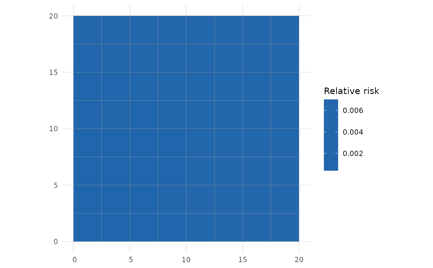
plot(pr, variable = "relative_risk")


## continuous surface on a grid
pr_c <- predict(fit, type = "continuous", cellsize = 1)
# }