Draws the latent field at the fitted optimum and returns posterior mean and SD of the incidence relative risk \(\exp(\mu+S)\) and covariate-adjusted relative risk \(\exp(S)\) for every region and time.
Usage
# S3 method for class 'SDALGCP2_ST'
predict(object, control.mcmc = NULL, ...)Value
a long sf of class
c("SDALGCP2_ST_pred", "sf", "data.frame") with one row per region and
time (ordered region-fastest within each time block) and columns
region, time, relative_risk, relative_risk_se
(\(\exp(\mu+S)\)), adjusted_rr and adjusted_rr_se
(\(\exp(S)\)) – the same column names as the spatial
predict.SDALGCP2. The posterior draws are kept in object
attributes (for exceedance); map a time slice with
plot.SDALGCP2_ST_pred.
Examples
# \donttest{
data(sdalgcp_data)
## stack the spatial example into a 3-time panel with a mild temporal trend
times <- 1:3
panel <- do.call(rbind, lapply(times, function(t) {
d <- sdalgcp_data; d$time <- t
d$cases <- rpois(nrow(d), d$pop * exp(-6 + 0.6 * d$x1 + 0.1 * (t - 2)))
d
}))
fit <- sdalgcp(cases ~ x1 + offset(log(pop)), data = panel, time = "time",
control = sdalgcp_control(n_sim = 2000, burnin = 500, thin = 5,
reanchor = 0))
pr <- predict(fit) # a long sf: region x time
head(pr)
#> Simple feature collection with 6 features and 6 fields
#> Geometry type: POLYGON
#> Dimension: XY
#> Bounding box: xmin: 0 ymin: 0 xmax: 15 ymax: 2.5
#> CRS: NA
#> region time relative_risk relative_risk_se adjusted_rr adjusted_rr_se
#> 1 1 1 0.0007198709 0.0002338193 1.1294531 0.3668546
#> 2 2 1 0.0007851638 0.0002428578 0.9615680 0.2974211
#> 3 3 1 0.0009492851 0.0003108810 0.9074499 0.2971804
#> 4 4 1 0.0013024469 0.0004173479 0.9718343 0.3114085
#> 5 5 1 0.0015708289 0.0004777553 0.9148866 0.2782556
#> 6 6 1 0.0016355303 0.0004621037 0.7435381 0.2100797
#> geometry
#> 1 POLYGON ((0 0, 2.5 0, 2.5 2...
#> 2 POLYGON ((2.5 0, 5 0, 5 2.5...
#> 3 POLYGON ((5 0, 7.5 0, 7.5 2...
#> 4 POLYGON ((7.5 0, 10 0, 10 2...
#> 5 POLYGON ((10 0, 12.5 0, 12....
#> 6 POLYGON ((12.5 0, 15 0, 15 ...
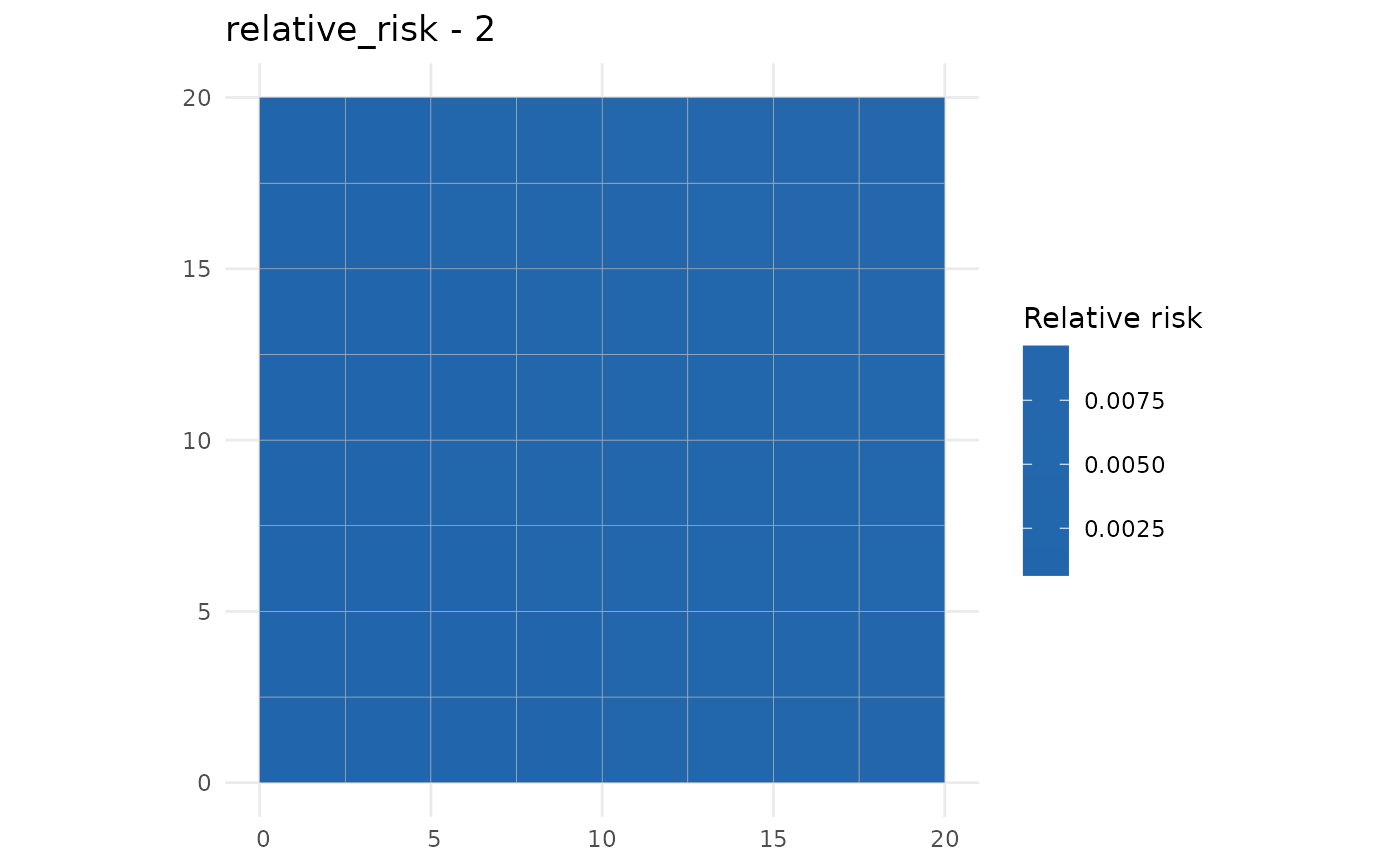
plot(pr, time = 2) # map the relative risk at time 2
 # }
# }